| EX | Model Training and Prediction |
In this exercise, we move from data preparation to the core of SDM: Model Training and Spatio-Temporal Prediction. We use a Random Forest (RF) classifier and address spatial autocorrelation using k-fold Nearest Neighbor Distance Matching (kNNDM) cross-validation.
1. Model Training
We begin by loading our presence/background data and environmental predictors. To ensure our model generalizes well to new geographic areas, we use the CAST package to create spatial folds.
Traditional random cross-validation often overestimates model performance because spatial data is inherently autocorrelated. knndm ensures that the distance between training and test points in the CV folds matches the distance between training data and the actual prediction domain.
library(CAST)
library(sf)
library(dplyr)


# 1 - load data ####
#------------------#

data=sf::read_sf("data/trainingData.gpkg")
po=data%>%dplyr::filter(presence==1)
bg=data%>%dplyr::filter(presence==0)

r=list.files("data/hyras_hessen/", pattern = "*.tif$", full.names = TRUE,
             recursive = TRUE)
r=terra::rast(r)

# 2 - create space time folds for cross-validation and testing ####
#-----------------------------------------------------------------#

KNNDMpo = CAST::knndm(tpoints = po, modeldomain = r,k=6)
po$KNNDM <- KNNDMpo$clusters
bg$KNNDM <- sample(1:6, nrow(bg), replace = TRUE)

data=rbind(po,bg);rm(po,bg,KNNDMpo)
data=na.omit(data)

# 4 -  ####
#------------------------

source("https://raw.githubusercontent.com/envima/sdmEvaluationMetrics/refs/heads/main/R/functions/rfModelTraining.R")

if(!dir.exists("data/output")) dir.create("data/output")
data$geom <- NULL


rf <- rfModelTraining(trainingData = data,
                      response = "presence",
                      spacevar = "KNNDM",
                      timevar = "time",
                     # variables = r,
                      k=5,
                      predictors= c("air_temp_max", "air_temp_mean", "photoperiod", "precipitation"),
                      outputPathModel = "data/output/phoenicurus_phoenicurus_rf.RDS",
                      prediction = FALSE)
Spatio-Temporal Prediction
Once the model is trained, we apply it to our raster stack. Since our predictors are time-specific (daily), we iterate through each date, rename the layers to match the model’s expected input, and generate a probability map.
library(terra)
library(dplyr)
library(tidyterra)
library(ggplot2)

# 1 - load data ####
#------------------#

RF = readRDS("data/output/phoenicurus_phoenicurus_rf.RDS")
r=list.files("data/hyras_hessen/", pattern = "*.tif$", full.names = TRUE,
             recursive = TRUE)
r=terra::rast(r)


# 1. Prepare Date metadata
# We extract the unique dates from your raster layer names
layer_names <- names(r)
# This regex extracts the 8-digit date string (e.g., 20260322)
dates <- unique(gsub(".*_", "", layer_names))

# 2. Iterate through each day and predict
results_list <- list()

for (d in dates) {
  cat("Processing date:", d, "\n")

  # Identify layers for the current date
  daily_layers <- grep(d, layer_names, value = TRUE)
  r_sub <- r[[daily_layers]]

  # CRITICAL: Rename layers to match the training names
  # Removes the "_YYYYMMDD" suffix so layers are named "air_temp_max", etc.
  names(r_sub) <- gsub(paste0("_", d), "", names(r_sub))

  # Ensure the model only sees the predictors it was trained on
  # (air_temp_max, air_temp_mean, photoperiod, precipitation)
  r_sub <- r_sub[[c("air_temp_max", "air_temp_mean", "photoperiod", "precipitation")]]

  # 3. Predict
  # Note: If your rf object is from the envima function,
  # it likely contains the caret/ranger model in rf$model or is the model itself.
  # Assuming rf is the trained model object:
  pred_day <- terra::predict(r_sub, RF, type = "prob", na.rm = TRUE)[[2]]
  names(pred_day)<-d
  # rescale raster between 0 and 1
  pred=climateStability::rescale0to1(pred_day)
  # Store or Save
  # It is usually safer to save each day to disk to avoid filling up RAM
  writeRaster(pred_day,
              filename = paste0("data/output/rf_", d, ".tif"),
              overwrite = TRUE)

  results_list[[d]] <- pred_day
}

# 4. (Optional) Create a Spatio-Temporal Raster Dataset
prediction_stack <- terra::rast(results_list)
terra::writeRaster(prediction_stack, "data/output/pred.tif")
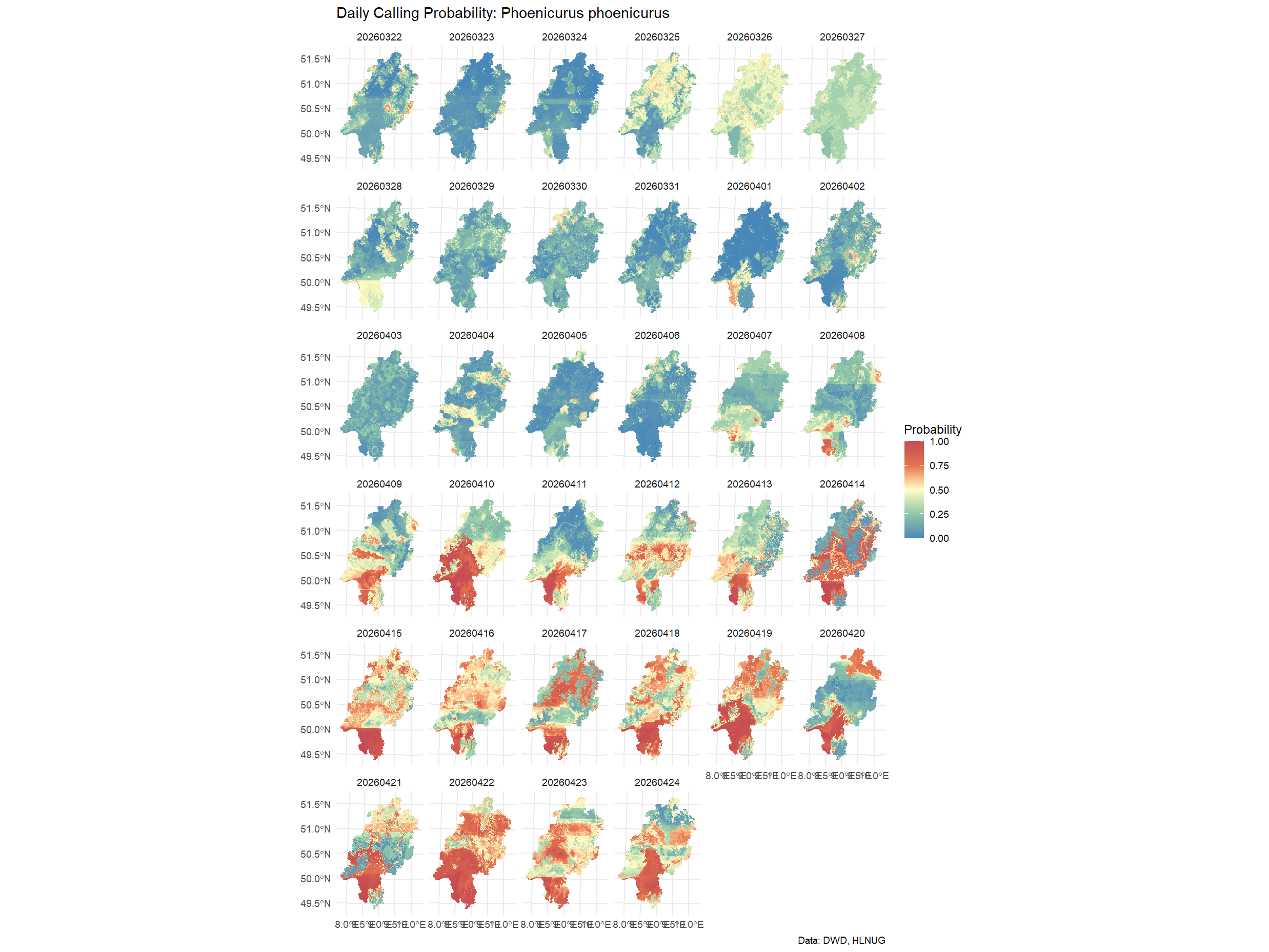
Visualizing Results
Visualizing the daily changes in occupancy probability allows us to identify phenological patterns or climate-driven shifts in the species’ distribution.
library(terra)
library(ggplot2)
library(tidyterra)

ggplot() +
  geom_spatraster(data = prediction_stack) +
  facet_wrap(~lyr) +
  scale_fill_whitebox_c(
    palette = "muted",
    limits = c(0, 1),
    name = "Probability"
  ) +
  theme_minimal() +
  labs(
    title = "Daily Calling Probability: Phoenicurus phoenicurus",
    caption = "Data: DWD, HLNUG"
  )