| EX | Bioacoustic and SDM |
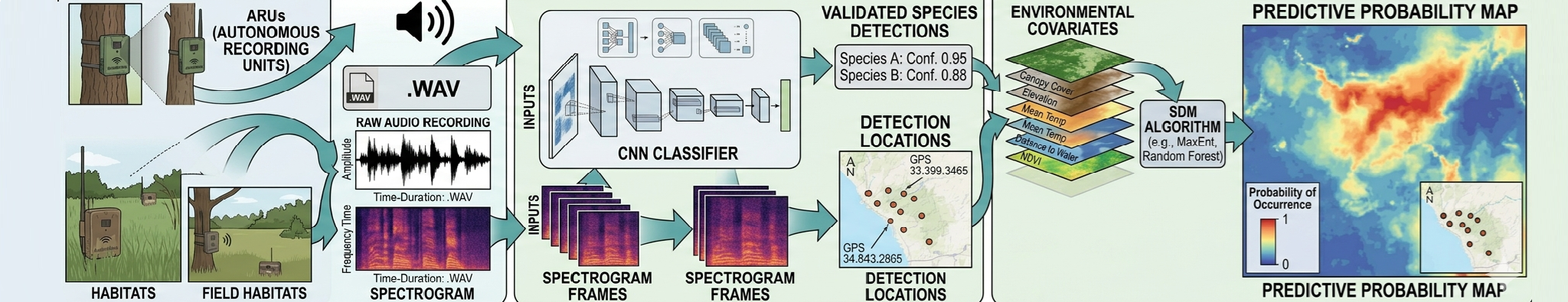
Species Distribution Modeling (SDM) utilizing bioacoustic data is a relatively new and evolving field. In this context, we don´t just model the spatial distribution of a species, but rather a calling probability. This approach is largely inspired by the research of Desjonquères et al. (2022), who modeled shifts in calling probability for a frog species on the Iberian Peninsula under climate change.
In this exercise, we will apply similar modeling techniques to a German bird species within the federal state of Hessen. However, rather than projecting future climate impacts, we will focus on seasonal dynamics, analyzing how calling probability fluctuates throughout the months based on environmental drivers.
From Detections to Occurance data
The primary output of bioacoustic monitoring is a “detection” (e.g., BirdNET confirms a Chaffinch was heard at 08:00 AM at station XYZ). In SDM, these detections have to be transformed to Presence-Only (or Presence-Absence) data. A significant challenge in this process is the sheer volume of data: a single station may record a Chaffinch every few seconds for several hours. Furthermore, each of these detections is associated with a specific confidence score from the classification model, typically on a scale from 0 to 1. Researchers must therefore define aggregation methods to convert these high-frequency, probabilistic detections into reliable occurrence points for spatial analysis.
On ILIAS, you can find a dataset of audio recordings collected on an edge device by trackIT Systems as part of the project Passive acoustic monitoring in bird sanctuaries in Hesse (german only) of the HLNUG (Hessian Agency for Nature Conservation, Environment and Geology). The project records with automatic recording devices on 65 stations in Hesse from 2026 to 2031 bird sanctuaries. We will use the first records of the project recorded from February to May 2026.
Read in the data and make yourself familiar with the structure:
library("dplyr")
library("sf")

data = sf::read_sf("data/gartenrotschwanz.gpkg")%>% rename(geometry = geom)
 Image: Phoenicurus phoenicurus by Jerzy Strzelecki. CC BY-SA 3.0.
,_Lodz_(Poland).jpg)
This dataset contains records for each station where the Phoenicurus phoenicurus (Common redstart) had beed recorded.
Environmental variables
To predict species distrbution or calling probability from acoustic data, detection records are combined with environmental variables. For this study, we primarily utilize meteorological data from the German Weather Service (DWD).
Using the provided script below, we download monthly grids for the year 2026, covering variables such as precipitation, air temperature, and solar radiation. These grids are cropped to the federal state of Hesse and processed at a spatial resolution of 1 km. This alignment allows us to correlate specific acoustic activity with the localized weather conditions present at each recording station.
# DWD HYRAS Daily Processing (2026 v6-1 only)
suppressPackageStartupMessages({
  library(terra)
  library(sf)
  library(geosphere)
  library(geodata)
})

# ---- Configuration -----------------------------------------------------------
project_root <- "C:/Users/bald_local/DATA/Lehre/moer-msc-advanced-SDM/data/aSDM/"
start_date   <- as.Date("2026-03-22")
end_date     <- as.Date("2026-04-24")

# Directories
out_dir_raw    <- file.path(project_root, "data/hyras_raw")
out_dir_hessen <- file.path(project_root, "data/hyras_hessen")
dir.create(out_dir_raw, recursive = TRUE, showWarnings = FALSE)
dir.create(out_dir_hessen, recursive = TRUE, showWarnings = FALSE)

# Product list (Only 2026 v6-1 files)
hyras_tasks <- list(
  precipitation = "https://opendata.dwd.de/climate_environment/CDC/grids_germany/daily/hyras_de/precipitation/pr_hyras_1_2026_v6-1_de.nc",
  air_temp_mean = "https://opendata.dwd.de/climate_environment/CDC/grids_germany/daily/hyras_de/air_temperature_mean/tas_hyras_1_2026_v6-1_de.nc",
  air_temp_max  = "https://opendata.dwd.de/climate_environment/CDC/grids_germany/daily/hyras_de/air_temperature_max/tasmax_hyras_1_2026_v6-1_de.nc"
)

# ---- Load Hessen -------------------------------------------------------------
message("Preparing Hessen boundary...")
hessen <- gadm(country = "DEU", level = 1, path = tempdir(), version = "latest")
hessen <- st_as_sf(hessen[grepl("hess", hessen$NAME_1, ignore.case = TRUE), ])

# ---- Processing Loop ---------------------------------------------------------
template_r <- NULL

for (prod_name in names(hyras_tasks)) {
  url <- hyras_tasks[[prod_name]]
  dest_file <- file.path(out_dir_raw, basename(url))

  # 1. Download
  if (!file.exists(dest_file)) {
    message("Downloading ", prod_name, "...")
    download.file(url, dest_file, mode = "wb", quiet = TRUE)
  }

  # 2. Load Raster
  r <- rast(dest_file)

  # 3. Time Filtering (Matching exact 2026 dates)
  time_vals <- time(r)
  indices   <- which(as.Date(time_vals) >= start_date & as.Date(time_vals) <= end_date)

  if (length(indices) == 0) {
    message("! Warning: No matching dates found in the file for ", prod_name)
    next
  }

  r_subset <- r[[indices]]

  # 4. Crop & Mask
  # Project Hessen vector to match the HYRAS NetCDF projection
  hessen_vect <- vect(st_transform(hessen, crs(r_subset)))
  r_hess <- mask(crop(r_subset, hessen_vect), hessen_vect)

  # 5. Metadata Cleanup
  # Ensure layer names reflect the variable and date
  names(r_hess) <- paste0(prod_name, "_", format(as.Date(time_vals[indices]), "%Y%m%d"))

  # 6. Save
  out_path <- file.path(out_dir_hessen, paste0("hessen_", prod_name, ".tif"))
  writeRaster(r_hess, out_path, overwrite = TRUE, gdal = c("COMPRESS=DEFLATE"))
  message("Successfully saved: ", out_path)

  # Keep first result as spatial template for photoperiod
  if (is.null(template_r)) template_r <- r_hess[[1]]
}

# ---- Photoperiod Predictor ---------------------------------------------------
if (!is.null(template_r)) {
  message("Generating daily photoperiod predictors for Hessen...")
  date_seq <- seq.Date(start_date, end_date, by = "day")

  # Calculate latitudinal daylength for each pixel
  xy <- xyFromCell(template_r, seq_len(ncell(template_r)))
  pts_lat <- st_coordinates(st_transform(st_as_sf(as.data.frame(xy), coords = c("x", "y"), crs = crs(template_r)), "EPSG:4326"))[, 2]

  ph_list <- lapply(date_seq, function(d) {
    doy <- as.integer(format(d, "%j"))
    setValues(template_r, geosphere::daylength(pts_lat, doy))
  })

  ph_stk <- rast(ph_list)
  names(ph_stk) <- paste0("photoperiod_", format(date_seq, "%Y%m%d"))
  writeRaster(ph_stk, file.path(out_dir_hessen, "hessen_photoperiod.tif"), overwrite = TRUE)
}

message("Full process complete. Daily 2026 data prepared for Hessen.")

Additional Environmental Variables
Beyond meteorological data, incorporating diverse environmental datasets can enhance the predictive power of an SDM or a calling probability model. High-resolution remote sensing data, in particular, is increasingly used to capture habitat characteristics (Regos et al. 2022, Randin et al. 2020).
Key environmental variables can be derived from the following sources:
- LiDAR Data: Used to quantify forest structure, including canopy height, vertical complexity, and understory density.
- Optical Remote Sensing: Satellite imagery provides spectral indices such as the Normalized Difference Vegetation Index (NDVI) to monitor vegetation health and phenology.
- Land Use Classifications: Useful for identifying specific habitat types, such as mixed forests, grasslands, or urbanized areas.
- Digital Elevation Models (DEM): Provide information on altitude, slope, and aspect, which affect local microclimates and species preferences.
If you wish to further refine your model, you may consider adding specific predictors such as NDVI derived from Landsat or Sentinel-2 data to account for seasonal changes in vegetation.
Creating a space-time dataframe
This exercise is a little bit different then the exemplary workflow in Unit 03 as we will not only predict general species distribution but calling probability at different times. This also means we need to do different data preprocessing as we need a dataframe with space-time information for model training. Furthermore, we also need to generate some kind of background information. Here we will use 10,000 randomly distributed background points for simplicity sake.
setwd("C:/Users/bald_local/DATA/Lehre/moer-msc-advanced-SDM/data/aSDM/")

library("dplyr")
library(terra)      # For raster handling
library(predicts)   # For background point sampling
library(sf)         # For spatial data frames
library(tidyverse)  # For data manipulation (dplyr, tidyr, stringr, purrr)
library(lubridate)
library(ggplot2)


data = sf::read_sf("data/gartenrotschwanz_full_data.gpkg")%>% rename(geometry = geom)


# Drop the geometry temporarily to speed up non-spatial grouping
data_summary <- data %>%
 # st_drop_geometry() %>%
  mutate(day = floor_date(time, "day")) %>%
  group_by(day, species, station) %>%
  summarise(
    n_detections = n(),
    mean_confidence = mean(confidence, na.rm = TRUE),
    .groups = "drop"
  )


library(quantreg)


q10 = quantile(data_summary$mean_confidence, probs = seq(0, 1, 0.1))[2][[1]]
y0 <- q10 # Your asymptote (the 10th percentile baseline)
a  <- 1 - q10 # The maximum penalty for n=1
med_n <- median(data_summary$n_detections) # The "pivot point" of your data
med_n<- quantile(data_summary$n_detections, 0.25)[[1]]
b_auto <- log(2) / med_n
# Define the threshold function
# As n increases, the required confidence drops toward 0.4
# $$C_{min}(n) = y_0 + a \cdot e^{-b \cdot n}$$$y_0$ (Asymptote):
#The baseline confidence you'd accept even if you have 10,000 detections (e.g., 0.42 based on your trend line).
#$a$ (Penalty): How much extra confidence you require for a single detection.
#$b$ (Decay): How fast you "forgive" the confidence requirement as more detections come in.


# 3. Define the automated function
threshold_curve <- function(n) {
  y0 + a * exp(-b_auto * n)
}

threshold_curve <- function(n) {
  q10 + (1-q10) * exp(-0.3 * n)
}

# Apply to your data
data_summary <- data_summary %>%
  mutate(
    req_confidence = threshold_curve(n_detections),
    is_reliable = mean_confidence >= req_confidence
  )


ggplot(data_summary, aes(x = n_detections, y = mean_confidence)) +
  geom_point(aes(color = is_reliable), alpha = 0.5) +
 # facet_wrap(~station)+
  scale_x_log10() +
  stat_function(fun = threshold_curve, color = "black", linewidth = 1, linetype = "dashed") +
  theme_minimal() +
  labs(title = "Exponential Filtering",
       subtitle = "Points above the dashed line are included")


data = data_summary%>%dplyr::filter(is_reliable == T);rm(data_summary)

sf::write_sf(data, "data/phoenicurus_phoenicurus_filtered_data.gpkg")
To filter the raw data we will use an exponential decay funtion that gradually filters out points with low confidence or with middle to low confidence and very little detections per day.
Creating a space time dataframe
Now we will create a dataframe with the extracted environmental data that contains information for each day. For each step in time we will also have one background dataset with 10,000 background points each.
setwd("C:/Users/bald_local/DATA/Lehre/moer-msc-advanced-SDM/data/aSDM/")

library("dplyr")
library(terra)      # For raster handling
library(predicts)   # For background point sampling
library(sf)         # For spatial data frames
library(tidyverse)  # For data manipulation (dplyr, tidyr, stringr, purrr)
library(lubridate)
library(ggplot2)


data = sf::read_sf("data/phoenicurus_phoenicurus_filtered_data.gpkg")%>% rename(geometry = geom)
data <- data %>%
  select(day,  station, geometry) %>%
  rename(time = day) %>%
  mutate(
    year  = year(time),
    month = month(time),
    day   = day(time),
    presence=1
  ) %>% sf::st_transform( sf::st_crs("EPSG:25832"))

#load the previously downloaded environmental variables

r=list.files("data/hyras_hessen/", pattern = "*.tif$", full.names = TRUE,
             recursive = TRUE)
r=terra::rast(r)

# Sample background points
bg = predicts::backgroundSample(mask = r[[1]], n = 10000)
bg = data.frame(bg)
bg = bg %>%
  sf::st_as_sf(coords = c("x", "y"), crs = st_crs(r)) %>%
  dplyr::mutate(presence = 0,station="bg")

# Get unique year/month pairs from your data
time_combos <- data %>%
  st_drop_geometry() %>%
  distinct(time, day, month, year)

# Create the cross-join (Every point x Every time step)
# This will result in (10,000 points * N time steps) rows
bg_expanded <- bg %>%
  cross_join(time_combos)


bg_expanded=sf::st_transform(bg_expanded, sf::st_crs("EPSG:25832"))

data = rbind(data,bg_expanded);rm(bg_expanded, bg, time_combos)

data = sf::st_transform(data, crs=terra::crs(r))

ext_matrix <- terra::extract(r, data, ID = FALSE)

# 2. Map the variables and dates
# Raster layer names look like: "air_temp_mean_20260322"
layer_names <- names(r)
# Extract the date part (YYYYMMDD) and the variable name part
raster_dates <- str_extract(layer_names, "\\d{8}$")
raster_vars  <- str_remove(layer_names, "_\\d{8}$")

# Unique variables (air_temp_max, air_temp_mean, photoperiod, precipitation)
unique_vars <- unique(raster_vars)

# 3. Match the 'data' dates to the 'raster' dates
# Create a YYYYMMDD string for each row in your data
data_date_strings <- format(data$time, "%Y%m%d")

# 4. Extract only the matching cells for each variable
# This loop avoids pivoting by pulling values directly from the extraction matrix
for(v in unique_vars) {
  message("Aligning variable: ", v)

  # Find which columns in 'ext_matrix' belong to this variable
  var_cols <- which(raster_vars == v)
  sub_matrix <- ext_matrix[, var_cols]
  colnames(sub_matrix) <- raster_dates[var_cols]

  # For each row in data, pick the column in the sub_matrix that matches data_date_strings
  # We use matrix indexing [row_index, col_index] for speed
  col_indices <- match(data_date_strings, colnames(sub_matrix))

  # Assign to data (using row/col indexing)
  data[[v]] <- sub_matrix[cbind(seq_len(nrow(data)), col_indices)]
}


# Remove the heavy matrix from memory
rm(ext_matrix)

sf::write_sf(data, "data/trainingData.gpkg")