
Checking Regression Assumptions
In the previous example, the Anscombe datasets had almost identical slopes and R² values but very different scatterplots. We now check whether the fitted lines and their F-tests are reasonable.
What do we need to check?
Recall the vertical segments in the regression plot: residual = observed − fitted. Their pattern helps us assess the model’s unobserved errors. The normality assumption concerns those errors, not the distribution of x or y alone.
Follow these checks in order. For each, describe what you see and what it means for the model. There is no separate submission.
| Question | How to check | What would raise a concern? |
|---|---|---|
| Does a straight line describe the mean response? | 1. Residuals versus fitted values | A systematic curve in the residuals, as for dataset 2 below. |
| Is the spread around the line roughly constant? | 2. Scale-location plot | Residuals become clearly more or less spread out. |
| Is a normal-error assumption plausible for the F-test? | 3. Residual QQ plot, then Shapiro–Wilk | Strong departures from the reference line. |
| Are observations independent? | 4. Sampling design | Repeated observations or related neighboring regions. |
Take-home message: Check residual patterns and sampling design before interpreting the slope test.
Prepare the models
Use all four Anscombe datasets from the previous page. This code recreates their models in a fresh R session. Each figure below shows datasets 1 and 2 in the top row, then 3 and 4 in the bottom row. In plot(), which selects the diagnostic view and main labels the dataset. Small numeric labels identify observations in the original data.
lmodels <- lapply(1:4, function(i) {
  lm(anscombe[, i+4] ~ anscombe[, i])
})
par_org <- par(no.readonly = TRUE)
Result: lmodels contains four fitted regressions, ready for the same diagnostic checks.
1. Check the mean pattern
The previous page plotted observed y against x: x on the horizontal axis and y on the vertical axis. Here, each observation becomes a point with its fitted y on the horizontal axis and its residual (observed − fitted) on the vertical axis. A positive residual means the observation lies above the fitted regression line; a negative residual means it lies below.
Look for residuals scattered around the horizontal zero line without a systematic curve. The red line summarizes the residual pattern; it is not the fitted regression line from the original scatterplot.
par(mfrow = c(2,2))
for(i in 1:4){
  plot(lmodels[[i]], which = 1, main = paste("Dataset", i))
}
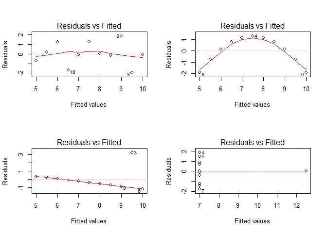
Read the top row first, then the bottom row:
- Dataset 1: residuals scatter around zero without a pronounced curve.
- Dataset 2: residuals are negative at both ends and positive in the middle. The straight-line model overestimates y at the ends and underestimates it in the middle: it misses the curved mean relationship.
- Dataset 3: one large positive residual stands out. That observation also pulls the fitted line away from the other points, leaving a pattern in their residuals. Investigate it rather than automatically deleting it.
- Dataset 4: ten points share x = 8, while one lies at x = 19. The fitted line passes exactly through that distant point, so its residual is zero. With only two x values, we cannot assess whether the mean relationship is straight or curved. The slope depends entirely on that one distant observation.
Take-home message: A suitable straight-line mean leaves no systematic curve in the residuals. The target here is scatter around zero, not points following a sloping line.
2. Check the spread
The scale-location plot shows residual sizes rescaled for comparison; it does not change the fitted model. Look for a roughly level red line and similar typical residual sizes across fitted values. A rising or falling pattern suggests changing error spread, which affects the usual F-test.
par(mfrow = c(2,2))
for(i in 1:4){
  plot(lmodels[[i]], which = 3, main = paste("Dataset", i))
}
## Warning: not plotting observations with leverage one:
##   8
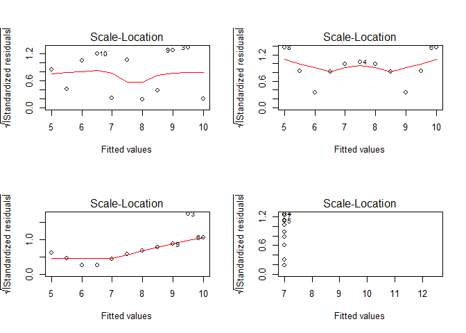
Dataset 1 has no obvious systematic spread change, but eleven observations provide limited evidence. In dataset 2, the curved mean distorts residual sizes; in dataset 3, the unusual observation affects the pattern. Neither provides a clean assessment of constant spread.
Dataset 4 cannot support a spread comparison across x: there is only one observation at x = 19. R warns that it cannot plot observation 8 with “leverage one”: the line is forced through that point, so its residual cannot be rescaled for this plot. It is also omitted from the QQ plot below; it remains in the fitted model.
Take-home message: Check the mean pattern first; changing residual spread is another reason to question the usual F-test.
3. Check the normal approximation
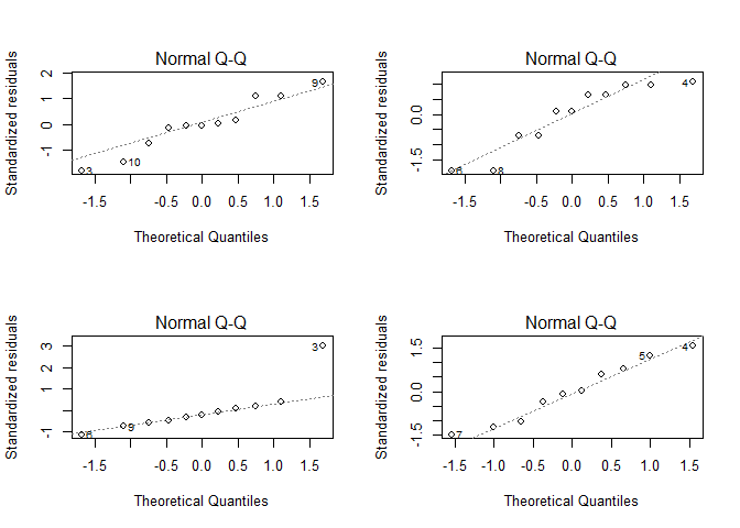
A normal QQ plot compares the residual pattern with what a normal distribution would produce. Points roughly following the reference line support this approximation; strong departures raise concerns. Check residuals, not raw x or y values.
par(mfrow = c(2,2))
for(i in 1:4){
  plot(lmodels[[i]], which = 2, main = paste("Dataset", i))
}
## Warning: not plotting observations with leverage one:
##   8
par(par_org)
Dataset 1 is reasonably close to the QQ reference line. Dataset 2 is visually borderline: its points show departures, but eleven observations give limited evidence about normality. Dataset 3 has a marked departure, consistent with its unusual observation. Dataset 4 shows no strong departure among the ten displayed residuals; the omitted distant point and limited x values still prevent an overall endorsement of the model.
Take-home message: A roughly straight QQ pattern supports a normal-error approximation; it does not confirm that the mean relationship is linear.
Add the Shapiro–Wilk test
The earlier ANOVA tested a zero slope. Shapiro–Wilk asks a different question: is the distribution normal? A p-value below 0.05 is evidence against normality; a larger value does not prove it. Use the test alongside the plots.
normality_p <- unlist(lapply(lmodels, function(model) {
  shapiro.test(residuals(model))$p.value
}))
data.frame(Dataset = 1:4, p_value = normality_p,
           Below_0.05 = normality_p < 0.05)
##   Dataset     p_value Below_0.05
## 1       1 0.545584685      FALSE
## 2       2 0.092948814      FALSE
## 3       3 0.001574055       TRUE
## 4       4 0.780048488      FALSE
Only dataset 3 falls below 0.05. Dataset 2 still needs a curved mean, despite its larger p-value. Small samples can hide departures; large samples can detect small ones. Fitted residuals share constraints from the estimated line, so treat these results as diagnostic indicators.
Take-home message: Read the p-value alongside the plots. Non-rejection does not establish that the model is adequate.
4. Check the sampling design
Independence means that observations do not share unexplained effects that link their errors. Recall Unit 04’s region and year identifiers: repeated measurements of one region, overlapping administrative areas or neighboring districts can be related. Selecting one year and one administrative level helps, but does not remove spatial dependence.
Take-home message: Independence needs support from the sampling design; a reassuring residual plot cannot establish it.
State your conclusion
Are the assumptions met? These small examples can reveal problems, but cannot prove that all assumptions hold. Independence is not established for any of the four datasets: these are constructed examples without a sampling design to assess.
| Dataset | What do the checks show? | Conclusion for the regression |
|---|---|---|
| 1 | No clear mean or spread problem; QQ pattern reasonably straight; Shapiro p ≈ 0.546. | Reasonably compatible with the assumptions checked by the plots. Minor irregularities with eleven observations are not clear violations. The usual slope test is reasonable if independence is justified. |
| 2 | Clear residual curve; spread assessment is confounded by the wrong mean shape. Normality is visually borderline; Shapiro p ≈ 0.093 does not reject at 0.05. | The straight-line mean assumption is not met. The borderline normality result does not rescue the model; do not rely on its usual slope test. |
| 3 | One unusual response distorts the fitted line and residual-size pattern. Strong QQ departure; Shapiro p ≈ 0.0016. | The normal-error assumption is not plausible for this fit. Investigate the unusual observation before relying on the usual slope test. |
| 4 | Mean shape and constant spread cannot be adequately checked across just two x values. QQ and Shapiro (p ≈ 0.780) show no strong normality warning. | The assumptions are not demonstrated. This is insufficient evidence, not proof of a violation. The slope rests on one distant point; avoid treating it as a well-supported general relationship. |
For Assignment 05, report the concern. No replacement model is required; do not remove observations or transform data just to make a test pass.
Take-home message: Connect the observed pattern → questionable assumption → consequence for your interpretation.
From one subset to Assignment 05
Forest vs. Agriculture applies these checks to the land-use table from Unit 04. It then asks whether the normality-test result changes across smaller samples.
First try one subset of Anscombe dataset 1: select eight rows, refit the model, and save the residual-test p-value. Selecting whole rows keeps the x–y pairs together.
set.seed(42)
chosen_rows <- sample(1:nrow(anscombe), size = 8, replace = FALSE)
one_sample <- anscombe[chosen_rows, ]
subset_model <- lm(one_sample$y1 ~ one_sample$x1)
subset_p <- shapiro.test(residuals(subset_model))$p.value
subset_p
## [1] 0.6140661
replace = FALSE prevents duplicates within this draw. set.seed() makes it reproducible in the same R setup; set it once before repeating draws and record the seed and R version. This subset’s p-value is above 0.05, so the test does not reject normality.
Repeat the workflow for the assignment’s 100 subsets of 50 districts. These subsets can overlap; they reuse the same observed data rather than providing new datasets.
Take-home message: The rejection frequency describes sensitivity to the selected samples, not the probability that the model is correct.
Here, fitting and diagnosis use the same rows. Unit 06 instead predicts held-out rows to assess prediction error.
References: R diagnostic plots, Shapiro–Wilk, NIST residual analysis.