
Example: Simple Bivariate Linear Regression
Linear regression modelling is one of the more common tasks in data analysis and the following example will cover the very basic topic of bivariate linear regression. The storyline follows the one from Zuur et al. (2007) to a certain degree.
While one could use actual data sets, we keep it controled by using an artificial data set originally compiled by Francis Anscombe. The anscombe dataset comes as part of base R. For now, we will use x1 as independent variable and y1 as dependent variable.
ind <- anscombe$x1
dep <- anscombe$y1
par_org <- par()
par(mfrow = c(1,2))
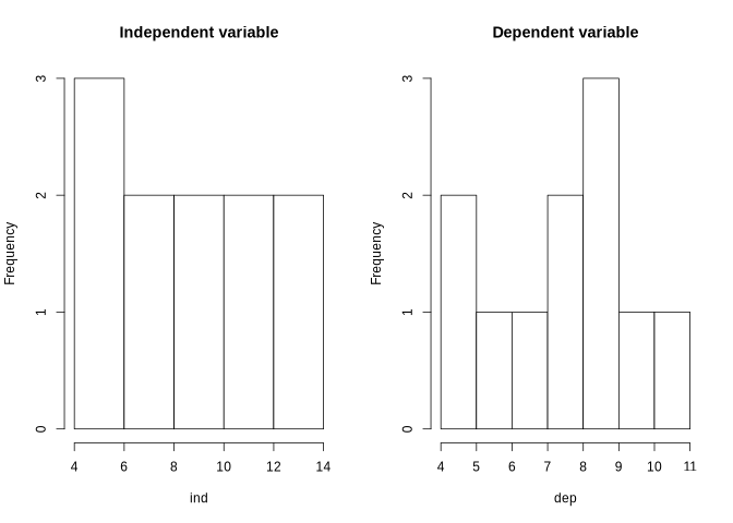
hist(ind, main = "Independent variable")
hist(dep, main = "Dependent variable")
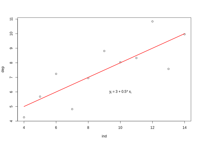
A look at the relationship between the variables by using a scatterplot justifies a linear modelling attempt. Fitting a bivariate linear model to the data set would result in the function shown in the plot and visualized by the red line.
library(car)
par(par_org)
plot(ind, dep)

lmod <- lm(dep ~ ind) # Compute linear regression model

regLine(lmod, col = "red") # Add regression line to plot (requires car package)
text(10, 6, bquote(paste("y"["i"], " = ", .(round(lmod$coefficients[1], 3)),
                          " + ", .(round(lmod$coefficients[2], 3)), "* x"["i"])))
While the visualization is illustrative, it does not provide any information on the actual significance of the parameters of the model, i.e. it does not answer the question after the existance of an actual linear relationship which - in the case of linear regression - requires a slope of the regression line which is actually different from 0. In principal, there are two ways to tackle this problem. Using an analysis of variance (ANOVA) or a t-test.
Testing a linear regression relationship by an analysis of variance
Let’s start with the ANOVA. In general, variance is the deviation of some value v from another value w for all pairs of v and w.
Given a (linear) model, each actual data value can be calculated by adding the fitted value and the corresponding residual value:
data value = fitted value + residual value (or y = y’ + res)
The associated variances are:
- The variance of the observed values, i.e. the difference between the individual observation y values and the mean over all observations of y. This will be called the observed (or total) variance.
- The variance of the fitted values, i.e. the difference between the predicted values of y’ and the mean over all observations of y. This will be called the model variance.
- The variance of the residual values, i.e. the difference between the predicted values y’ and the observed values y. This will be called the residual variance.
The sum of model variance and residual variance equals the observed variance.
Commonly, all variances are squared and summed up over all observations which gives us the observed sum of squares, the model sum of squares and the residual sum of squares.
In order to calculate the variances, one can use the lm class of the model since - among others - it contains the original independent and dependent values as well as the predicted ones:
ss_obsrv <- sum((lmod$model$dep - mean(lmod$model$dep))**2)
ss_model <- sum((lmod$fitted.values - mean(lmod$model$dep))**2)
ss_resid <- sum((lmod$model$dep - lmod$fitted.values)**2)
Since the sum increases with increasing numbers of observations, the resulting sum of squares are normalized by the respective degrees of freedom. This gives us:
- the mean observed sum of squares
- the mean model sum of squares
- the mean residual sum of squares, i.e. the mean squared error if the model is a simple linear regression model.
mss_obsrv <- ss_obsrv / (length(lmod$model$dep) - 1)
mss_model <- ss_model / 1
mss_resid <- ss_resid / (length(lmod$model$dep) - 2)
It can be shown that for large sample sizes, the mean residual sum of squares equals the squared variance of the population. In this case, the mean model sum of squares equals the squared variance of the population plus the sum of squares over all x values multiplied by the slope of the regression model. In other words,
- if the slope is zero, then mean model sum of squares and mean residual sum of squares are equal and the ratio of both is 1.
- if the slope is not zero, then mean model sum of squares is larger than the mean residual sum of squares and the ratio is larger than 1.
This provides us the test statistic for the null-hypothesis that the true slope is not different from 0.
f_value <- mss_model / mss_resid
The F-statistic quantifies how much larger the variation explained by the model is compared to the variation left unexplained (residuals).
- A large F value indicates that the model explains a lot more variation than is left unexplained, suggesting that the slope is likely not 0.
- A small F value indicates that the model doesn’t explain much more variation than the residuals, suggesting that the slope might be 0.
By comparing the computed F value to an F distribution with 1 numerator degree of freedom and (number of observations - 2) denominator degrees of freedom, the p value is determined. If the p value is very small, the null-hypothesis can be rejected.
p_value <- pf(f_value, 1, length(dep) - 2, lower.tail = FALSE)
In summary, this gives us the following:
data.frame(Name = c("ind", "residuals"),
           Deg_of_freedom = c(1, length(lmod$model$dep) - 2),
           Sum_of_squares = c(ss_model, ss_resid),
           Mean_sum_of_squares = c(mss_model, mss_resid),
           F_value = f_value,
           p_value = p_value)
##        Name Deg_of_freedom Sum_of_squares Mean_sum_of_squares  F_value
## 1       ind              1       27.51000           27.510001 17.98994
## 2 residuals              9       13.76269            1.529188 17.98994
##       p_value
## 1 0.002169629
## 2 0.002169629
Of course, one does not have to compute this every time. A simple call to the anova function will do it:
anova(lmod)
## Analysis of Variance Table
##
## Response: dep
##           Df Sum Sq Mean Sq F value  Pr(>F)
## ind        1 27.510 27.5100   17.99 0.00217 **
## Residuals  9 13.763  1.5292
## ---
## Signif. codes:  0 '***' 0.001 '**' 0.01 '*' 0.05 '.' 0.1 ' ' 1
Exercise. Now you can check your knowledge and strengthen your plotting skills by writing code to rebuild the linear regression scatterplot from the previous page. When coding, think about the meaning of slope, intercept, observed variance, model variance, residual variance, and the different types of sum of squares.
R squared
The variance explained by the model is one of the most often used variables to explain the relationship in simple linear models. It is computed by normalizing either the model sum of squares by the observed sum of squares or by substracting the normalization of the residual sum of squares from 1.
ss_model / ss_obsrv
## [1] 0.6665425
1 - ss_resid / ss_obsrv
## [1] 0.6665425
Convention. p and r-squared often denote results of bivariate linear regressions while P and R-squared (capital letters) often denote results of multiple linear regressions. The letters p (P) and r2 (R2) are often written in italics.
Finished?
Well, the above looks like a real good example of linear regression analysis, right? And the r-squared of about 0.67 is also quite OK not to mention the significance of the independent variable.
Before we clap our hands, let’s just have a look at the other variable combinations of the Anscombe data set.
par(mfrow = c(2,2))
for(i in seq(4)){
  plot(anscombe[, i], anscombe[, i+4],
       xlab = names(anscombe[i]), ylab = names(anscombe[i+4]))
}
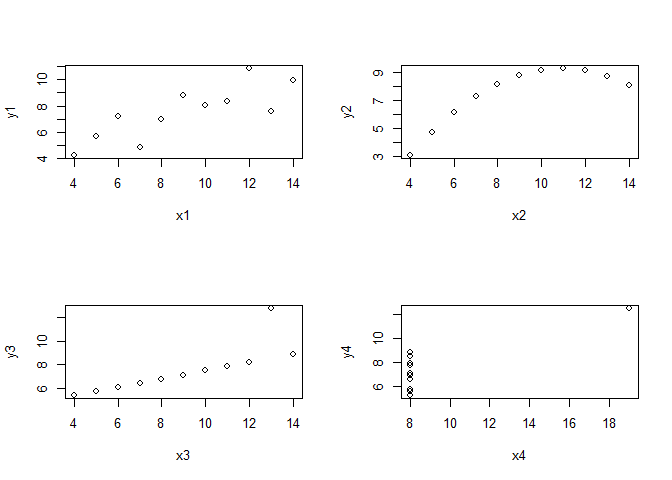
While x3/y3 might still justify a linear regression if we remove the outlier, the two plots on the right side do not. So what to do? Unfortunately, all of these data combinations result in almost the same regression statistics:
lmodels <- lapply(seq(4), function(i){
  lm(anscombe[, i+4] ~ anscombe[, i])
})
lapply(lmodels, summary)
## [[1]]
##
## Call:
## lm(formula = anscombe[, i + 4] ~ anscombe[, i])
##
## Residuals:
##      Min       1Q   Median       3Q      Max
## -1.92127 -0.45577 -0.04136  0.70941  1.83882
##
## Coefficients:
##               Estimate Std. Error t value Pr(>|t|)
## (Intercept)     3.0001     1.1247   2.667  0.02573 *
## anscombe[, i]   0.5001     0.1179   4.241  0.00217 **
## ---
## Signif. codes:  0 '***' 0.001 '**' 0.01 '*' 0.05 '.' 0.1 ' ' 1
##
## Residual standard error: 1.237 on 9 degrees of freedom
## Multiple R-squared:  0.6665,	Adjusted R-squared:  0.6295
## F-statistic: 17.99 on 1 and 9 DF,  p-value: 0.00217
##
##
## [[2]]
##
## Call:
## lm(formula = anscombe[, i + 4] ~ anscombe[, i])
##
## Residuals:
##     Min      1Q  Median      3Q     Max
## -1.9009 -0.7609  0.1291  0.9491  1.2691
##
## Coefficients:
##               Estimate Std. Error t value Pr(>|t|)
## (Intercept)      3.001      1.125   2.667  0.02576 *
## anscombe[, i]    0.500      0.118   4.239  0.00218 **
## ---
## Signif. codes:  0 '***' 0.001 '**' 0.01 '*' 0.05 '.' 0.1 ' ' 1
##
## Residual standard error: 1.237 on 9 degrees of freedom
## Multiple R-squared:  0.6662,	Adjusted R-squared:  0.6292
## F-statistic: 17.97 on 1 and 9 DF,  p-value: 0.002179
##
##
## [[3]]
##
## Call:
## lm(formula = anscombe[, i + 4] ~ anscombe[, i])
##
## Residuals:
##     Min      1Q  Median      3Q     Max
## -1.1586 -0.6146 -0.2303  0.1540  3.2411
##
## Coefficients:
##               Estimate Std. Error t value Pr(>|t|)
## (Intercept)     3.0025     1.1245   2.670  0.02562 *
## anscombe[, i]   0.4997     0.1179   4.239  0.00218 **
## ---
## Signif. codes:  0 '***' 0.001 '**' 0.01 '*' 0.05 '.' 0.1 ' ' 1
##
## Residual standard error: 1.236 on 9 degrees of freedom
## Multiple R-squared:  0.6663,	Adjusted R-squared:  0.6292
## F-statistic: 17.97 on 1 and 9 DF,  p-value: 0.002176
##
##
## [[4]]
##
## Call:
## lm(formula = anscombe[, i + 4] ~ anscombe[, i])
##
## Residuals:
##    Min     1Q Median     3Q    Max
## -1.751 -0.831  0.000  0.809  1.839
##
## Coefficients:
##               Estimate Std. Error t value Pr(>|t|)
## (Intercept)     3.0017     1.1239   2.671  0.02559 *
## anscombe[, i]   0.4999     0.1178   4.243  0.00216 **
## ---
## Signif. codes:  0 '***' 0.001 '**' 0.01 '*' 0.05 '.' 0.1 ' ' 1
##
## Residual standard error: 1.236 on 9 degrees of freedom
## Multiple R-squared:  0.6667,	Adjusted R-squared:  0.6297
## F-statistic:    18 on 1 and 9 DF,  p-value: 0.002165
So be careful when interpreting p and R-squared values! We will learn how to treat non-linear relationships in the subsequent units.
Minimum assumption(s) for bivariate linear regression models
The above example illustrates why it is important to understand a concept and not just to know how something is computed. In the present example, we have to make some additional checks, which give us information about the distribution of variables in order to actually decide if we want to do some assessments based on e.g. the retrieved r-squared value.
The following checks are what should at least be considerd in bivariate linear regression (for multiple linear regression, multicollinearity of the independent variables is crucial):
- homogeneity of the variance of residuals (homoscedasticity)
- normality of the residuals (much less important, but handy for small samples)
The normality of the residuals could be checked by normality tests but these tests do not prove normality but test the null-hypothesis that something is not normal. E.g. a Shapiro-Wilk normality test with an insignificant p value does not reject the hypothesis that the distribution is normal but it does not prove that the distribution is actually normal. In addition, for small data, such tests often fail to reject non-normal distributions while for large samples, even very small deviations with no fundamental implication on e.g. anova results lead to a rejection. Speaking about anova influences: anovas are quite robust against violations of normality. For now, we will restrict our evaluation of the model to a visual approach.
Let’s start with the most important assumption, the one of homogeneous variances in the residuals, aka the homoscedasticity:
par(par_org)
par(mfrow = c(2,2))
for(i in seq(4)){
  plot(lmodels[[i]], which = 1)
}
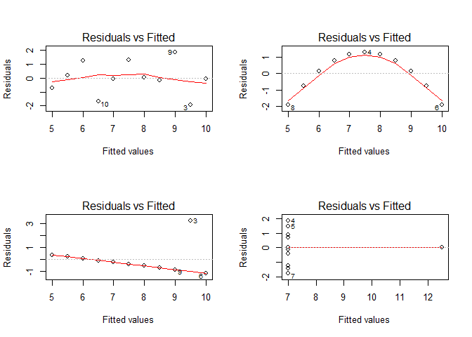
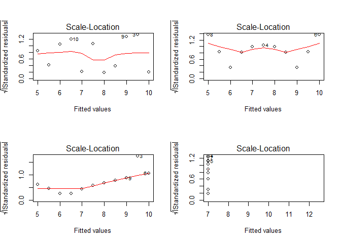
Except maybe for the upper left figure, this assumption is clearly violated as can be shown on residuals vs. fitted values plots. A better visualization might be the scale-location plot which standardizes the residuals and performs a square-root transformation on them. In doing so, the variance of the residuals becomes more evident in the case of small deviations from the homoscedasticity assumption:
par(mfrow = c(2,2))
for(i in seq(4)){
  plot(lmodels[[i]], which = 3)
}
If you want to check the normality of the residuals, we could visualize their distribution as a QQ plot.
par(mfrow = c(2,2))
for(i in seq(4)){
  plot(lmodels[[i]], which = 2)
}
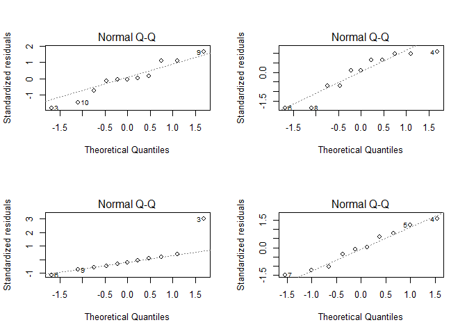
par(par_org)
Also there are deviations from a straight line, the deviations except for the lower left plot are not really crucial (and there it is only for the data pair labled with 3). The lower left plot is also the only plot where the Shapiro-Wilk test rejects the normal distribution hypothesis on a p < 0.05 level.
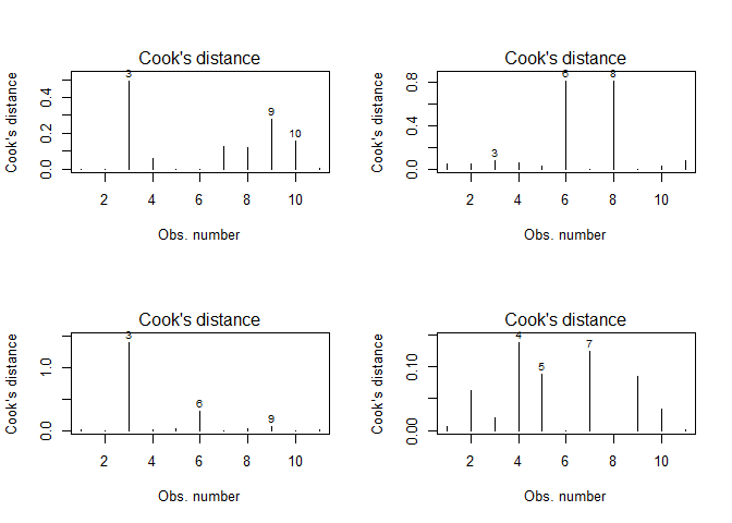
You might wonder why some of the points in the above figures are labled (e.g. 3, 9, 10 in the upper left plots). These numbers in the plots refer to the observation number in the original dataset. This feature results from an “influential points analysis” using Cook’s distance, which is a measure of how strong the regression parameters change if a certain observation is not considered. Hence, the larger this change, the larger the influence of this particular observation. For the above data, Cook’s distance looks like that:
par(mfrow = c(2,2))
for(i in seq(4)){
  plot(lmodels[[i]], which = 4)
}
No alternatives?
In case that your linear regression assessment shows some violations, the end is not to come, yet. According to Zuur et al. (2007), the solutions to common problems are the following:
- Violation of homogeneity (residuals vs. fitted values plot) without a pattern in the residual vs. observations (i.e. x values) plot: transform the y values or use generalized models
- Violation of homogeneity (residuals vs. fitted values plot) with a pattern in the residual vs. observations (i.e. x values) plot: add non-linear terms of the independent variable
- No violation of homogeneity (residuals vs. fitted values plot) but a pattern in the residual vs. observations (i.e. x values) plot: transform the x values or use additive modelling
Before transforming your variables beyond recognition think about if you really need a linear regression for your data analysis task. In doubt use some other statistical method like generalized additive models.