For-loops
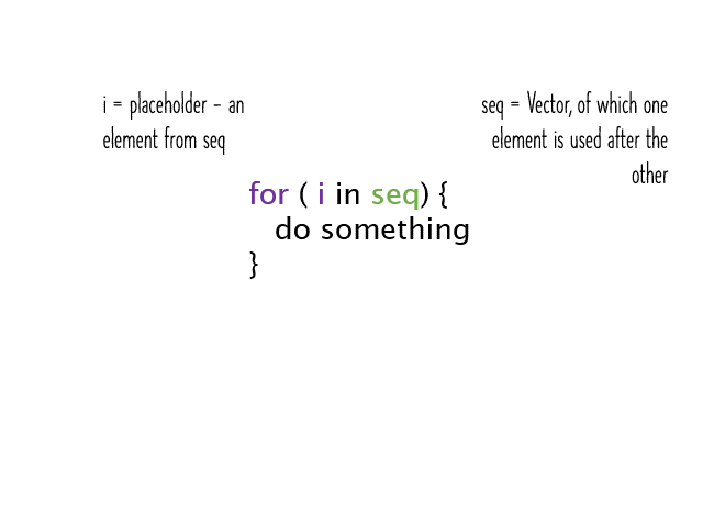
For-loops are the mother of all repeating structures which enable the execution of certain code blocks for multiple times. For-loops are useful if the number of necessary repetitions is known at the starting time of the loop (which is not necessarily the starting time of the program!).
In for loops, the number of repeated executions is given at the start time either by a variable which is defined during the runtime of the previous code or by a constant supplied by the programmer. Imaging that we know already how many times the loop has to be repeated, one can implement it simply as:
for(i in seq(7,10)){
  print(i)
}
## [1] 7
## [1] 8
## [1] 9
## [1] 10
Note that the variable i which controls the for loop must not be changed within the loop.
Of course, you can nest for loops:
for(i in seq(7, 10)){
  print(paste0("Outer loop value of a: ", i))
  if(i < 10){
    lower_border <- i + 1
  } else {
    lower_border <- i
  }
  for(j in seq(10, lower_border)){
    print(paste0("   Inner loop value of c: ", j))
  }
}
## [1] "Outer loop value of a: 7"
## [1] "   Inner loop value of c: 10"
## [1] "   Inner loop value of c: 9"
## [1] "   Inner loop value of c: 8"
## [1] "Outer loop value of a: 8"
## [1] "   Inner loop value of c: 10"
## [1] "   Inner loop value of c: 9"
## [1] "Outer loop value of a: 9"
## [1] "   Inner loop value of c: 10"
## [1] "Outer loop value of a: 10"
## [1] "   Inner loop value of c: 10"
The loop might look complicated but the reason for that is just the if-else statement. It is necessary since the second loop must run from c to the integer value just larger than a (i.e. 8, 9, 10). Therefore, a must be increased by 1 if it is smaller than 10 but stay 10 if it equals 10.
Instead of defining the number of repetitions in the for loop statement, one can also use any vector variable. The number of iterations will always be equal to the length of the vector. This is not surprising, since the seq function used so far also simply returns a vector, e.g.:
t <- seq(7, 10)
t
## [1] 7 8 9 10
class(t)
## [1] "integer"
As obvious from the above examples, the iteration variable (i.e. i or j in our examples above ) is set to the first value of the vector during the first iteration, then to the second value during the second iteration and so on. Since the number of repititions is defined by the length of the control vector and not by the values within it, one can also use a vector with e.g. characters to construct a for loop:
a <- c("A", "B", "C", "D")
for(elements in a){
  print(elements)
}
## [1] "A"
## [1] "B"
## [1] "C"
## [1] "D"
Important: while this behaviour is usefull for programming pros, it might be very confusing for greenhorns. Therefore you can just stick to using numbers as iteration elements. The above for loop can be implemented using numbers as follows:
for(i in seq(4)){
  print(a[i])
}
## [1] "A"
## [1] "B"
## [1] "C"
## [1] "D"
If you want to use this for arbitrary lengths of vector a, just pass the length of the vector into the seq function:
for(i in seq(length(a))){
  print(a[i])
}
## [1] "A"
## [1] "B"
## [1] "C"
## [1] "D"
Modifying an existing variable in a loop
If you want to modify a existing variable, for (and while) loops are the only option (i.e. you can not use lapply). Aside from that restriction, it is a straight forward task. Let’s just add an “x” to each entry of variable a:
a <- c("A", "B", "C", "D")
for(i in seq(length(a))){
  a[i] <- paste0(a[i], "x")
}
a
## [1] "Ax" "Bx" "Cx" "Dx"
If you want to get some feedback for each iteration while a loop is running, try to add a line like:
cat("Current iterator: ", i, " | ", "Current content of object: ", a, "\n", sep = "")
Of course the same is possible for data frames. Let’s make an example where we have the following data frame:
a <- c("A", "B", "C", "A", "B", "A", "A")
b <- c("X", "X", "X", "X", "Y", "Y", "Y")
c <- c(1, 2, 3, 4, 5, 6, 7)
d <- c(10, 20, 30, 40, 50, 60, 70)
df <- data.frame(Cat1 = a, Cat2 = b, Val1 = c, Val2 = d)
We now want to modify this data frame in that way that the characters of columns Cat1 and Cat2 are converted to lower case and the values of Val1 and Val2 are converted to their square root. Therefore we must iterate over each column and then we can apply the lowercase function to all rows of the first two columns and the sqrt function to all entries of the last two columns. While we could use seq(4) as control vector, we can also get the number of columns from the data frame using the ncol function:
for(i in seq(ncol(df))){
  if(is.factor(df[,i])){
    df[,i] <- tolower(df[,i])
    } else if(is.numeric(df[,i])){
      df[,i] <- sqrt(df[,i])
      }
  }
As you can see, we iterate over the columns of the data frame by using i as column index (i.e. df[,i]). If the actual column is a factor (first if statement), the content of the actual column is converted to lower cases and the original
column content is overwritten (line 3). If the actual column is numeric (second if statement), the content of this column is converted to its square root and the original column content is overwritten (line 4).
In the end, the data frame looks like this:
df

##   Cat1  Cat2    Val1     Val2
## 1    a    x   1.000000   3.162278
## 2    b    x   1.414214   4.472136
## 3    c    x   1.732051   5.477226
## 4    a    x   2.000000   6.324555
## 5    b    y   2.236068   7.071068
## 6    a    y   2.449490   7.745967
## 7    a    y   2.645751   8.366600
Building a new variable with a loop
The above examples show how to modify an existing variable. If you want to keep your original values but safe the results in a new variable, you have to define it first outside the loop. Afterwards you modify it within the loop so it is similar to the task above.
For example, if you want to convert the elements of vector a to lower case and store the results in another vector, the following would be necessary:
test <- character()   # this is an empty character vector
for(i in seq(length(a))){
  test <- c(test, tolower(a[i]))
}

test

## [1] "a" "b" "c" "a" "b" "a" "a"
Please note that this example can of course easily implemented without a loop so just take it as a simple illustration.
If you want to construct a data frame, it is just a little more complicated. Let’s get back to the original data frame used in the example just above:
a <- c("A", "B", "C", "A", "B", "A", "A")
b <- c("X", "X", "X", "X", "Y", "Y", "Y")
c <- c(1, 2, 3, 4, 5, 6, 7)
d <- c(10, 20, 30, 40, 50, 60, 70)
df <- data.frame(Cat1 = a, Cat2 = b, Val1 = c, Val2 = d)
If the lowercase/square root conversion results should be stored in a new data frame, we have to define at least one column of this new data frame first:
df_new <- data.frame(Col1 = rep(NA, nrow(df)))

df_new

##   Col1
## 1   NA
## 2   NA
## 3   NA
## 4   NA
## 5   NA
## 6   NA
## 7   NA
We simply initialize the column with so many rows as we find in the source data frame (i.e. nrow(df)). Since one can not initialize a completely empty column, we write NAs in it.
Let’s start with the loop:
for(i in seq(ncol(df))){
  if(is.factor(df[,i])){
    df_new[,i] <- tolower(df[,i])
    } else if(is.numeric(df[,i])){
      df_new[,i] <- sqrt(df[,i])
      }
  }
The only difference to the example above is that the result of the conversions are not stored in the original data frame but in our newly created one. Let’s have a look at its content:
df_new

##   Col1 V2       V3       V4
## 1    a  x 1.000000 3.162278
## 2    b  x 1.414214 4.472136
## 3    c  x 1.732051 5.477226
## 4    a  x 2.000000 6.324555
## 5    b  y 2.236068 7.071068
## 6    a  y 2.449490 7.745967
## 7    a  y 2.645751 8.366600
Looks good. Obviously, columns two to four (i.e. V2, V3, V4) have been created automatically when i in df_new[,i] was 2, 3 or 4.
If you want to change the column names to the original column names of data frame df, just do it:
colnames(df_new) <- colnames(df)
str(df_new)
## 'data.frame':	7 obs. of  4 variables:
##  $ Cat1: chr  "a" "b" "c" "a" ...
##  $ Cat2: chr  "x" "x" "x" "x" ...
##  $ Val1: num  1 1.41 1.73 2 2.24 ...
##  $ Val2: num  3.16 4.47 5.48 6.32 7.07 ...
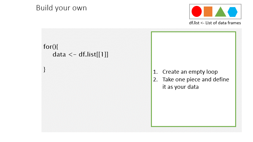
DIY loops - some tipps
Sometimes it can be a little overwhelming to write a loop from top to bottom. That’s why it makes sense to tackle the whole thing piece by piece. The following approach might be helpful.
1) Start by setting up an empty for(){} loop, establishing the structure for your iterative process. This initial step helps maintain proper text indentation and structure in your code.
2) Take one piece of your data and define it as your data source.
3) Write down all the operations you want to perform within the loop.
4) Identify and handle replaceable elements within your loop. These are parts of your code that may change during each iteration. Use variables or placeholders to represent these elements, enhancing code flexibility and readability.
5) Think about how you want to save the output of each iteration. Create a result container, such as a list or matrix, outside the loop, and store the results there.
6) Consider using vectorized operations when possible to improve loop efficiency and reduce code complexity.
7) Debug and test your loop incrementally, checking for errors and unexpected behavior after each iteration. Depending on the complexity of the data, the loop may not be complete. Missing data, for example, often leads to a subscript out of bound error. To eliminate these errors bit by bit, you can use the cat(i,”\n”) command to specify the point at which the loop stops, and continue to process the data or add conditions accordingly.