Object Types
You may like to store information of various data types like character, integer, floating point, Boolean etc. Based on the data type of a object, the operating system allocates memory and decides what can be stored in the reserved memory.
The objects are assigned with R-Objects and the data type of the R-object becomes the data type of the object. There are many types of R-objects. The frequently used ones are:
- Vectors
- Data Frames
- Matrices
- Arrays
- Lists
- Factors
The simplest of these objects is the vector object and there are six data types of these atomic vectors, also termed as six classes of vectors. The other R-Objects are built upon the atomic vectors.
| Data Type in R | Example | Data Type from previous lesson |
|---|---|---|
| integer | 1; 15 ; 1984297 | int |
| numeric | 1.15 ; 1007.28 ; 0.0001 | float |
| character | © ; H ; π ; “Hello World” ; “Ursus maritimus” ; “black” | character combines character and strings |
| logical | true ; false | boolean |
Objects
Objects are the core of any R program. They contain the information we calculate with and also the calculated results. They also offer the possibility to label data with meaningful names, so that the code is easier to understand. It is helpful to think of objects as containers that hold information. Their sole purpose is to label and store data which then can be used across the code.
How to name an object?
“All things are defined by names. Change the name, and you change the thing” — Terry Pratchett, Pyramids
Even though data is very diverse, objects cannot take every name. This is because they must be unique to the computer. They can contain letters, numbers and underscores ( _ ), though the latter cannot be used at the beginning of the name. All other characters and spaces are not allowed. This restriction is important because R has to understand the input data, furthermore it has to be unique for the program. For example, if minus signs (-) were allowed for naming (which they are not!), there would be an ambiguity with the name all-animals. R would not know whether we meant the object all-animals or whether we wanted to subtract the object animals from the object all.
Instead, we could call it all_animals, AllAnimals, allanimals, Allanimals or allAnimals.
Note that R distinguishes between upper and lower case for names. allAnimals and AllAnimals are not the same object and it is not possible to switch them.
You should generally not use names, which are reserved for functions (e.g mean). Try to find meaningful names, but try to make them relatively short, too.
How to define objects?
The assignment operator looks like an arrow (<-) and is used to assign values to objects. It is built through a smaller-than (or greater-than)-symbol and a minus. In R there are several possibilities to define an object:
# Assign the value y to object x
x <- value_y
value_y -> x
These two do the same: they assign a value to the object x, but the first variant is used much more often than the second.
Second Example:
# Assign the value "Hello World" to object "greeting"
greeting <- "Hello World."

#show content of object "greeting"
greeting
[1] Hello World.
You could also use the “=” sign to assign objects. However, the = operator is conventionally used to specify named arguments in function calls. To avoid ambiguity and potential conflicts between function argument names and object names, using <- for assignment helps reduce the chance of errors.
Vectors
If you want to store more than one value to an object you need a vector. It is a basic data structure and contains elements of the same type. The data types can be logical, integer, double and character.
When you want to create a vector with more than one element, you need to use the c() function which means to combine the elements into a vector (c for combine).
apple <- c("red", "green","yellow")
apple

[1] "red"    "green"  "yellow"
A vector’s type can be checked with the typeof() function. apple is a word not a number therefore it is a character (in other words a string).
# Ask for the class of the vector
apple <- c("red", "green","yellow")
typeof(apple)

[1] "character"
Another important property of a vector is its length. This is the number of elements in the vector and can be checked with the function length(). In this case the length is 3. Three Values for “red”, “green” and “yellow”.
#Ask for the length of the vector
apple <- c("red", "green","yellow")
length(apple)

[1] 3
A vector can only contain values of the same data type.
You can add elements, again by using c()
#add an element
apple <- c(apple, "brown")
apple

[1] "red"    "green"  "yellow"   "brown"
If needed, you can also assign names to the single elements:
#add names
names(apple) <- c("Col1","Col2","Col3","Col4")
apple

 Col1       Col2      Col3      Col4
"red"    "green"  "yellow"   "brown"
If you need to repeat an element of a vector several times, you can use the rep()-function:
#repeat
applebucket <- rep(apple,3)
applebucket

    Col1     Col2     Col3     Col4     Col1     Col2     Col3     Col4
   "red"  "green" "yellow"  "brown"    "red"  "green" "yellow"  "brown"
    Col1     Col2     Col3     Col4
   "red"  "green" "yellow"  "brown"
The whole vector is repeated three times. Check the arguments of ?rep to find a way of repeating each element in the vector three times.
vectorization
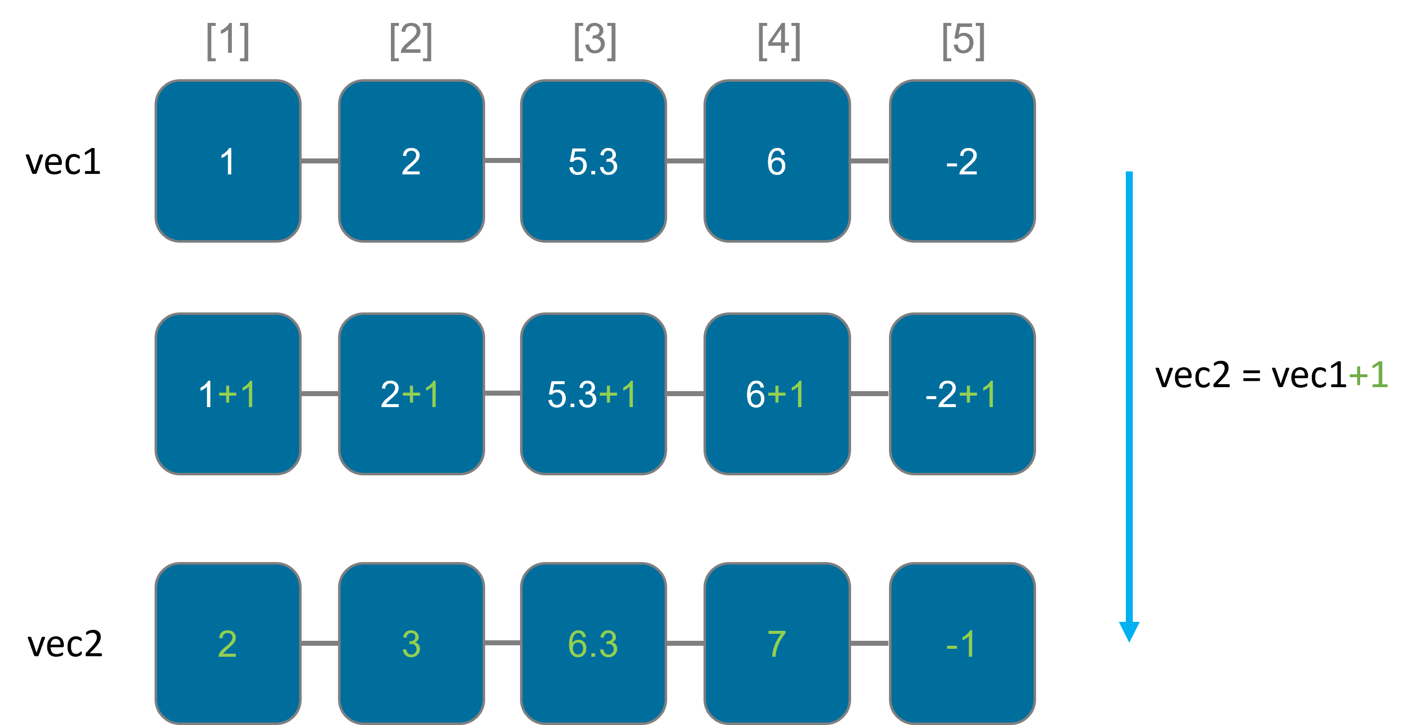
In R, most (but not all!) functions are automatically applied to all elements of a vector.

When you perform an operation on two vectors of the same length, R will automatically apply the operation element-wise, meaning it performs the operation between the corresponding elements of the vectors
x <- c(1,2,3)
y <- c(4,5,6)
result <- x+y
result
[1] 5,7,9
Recycling
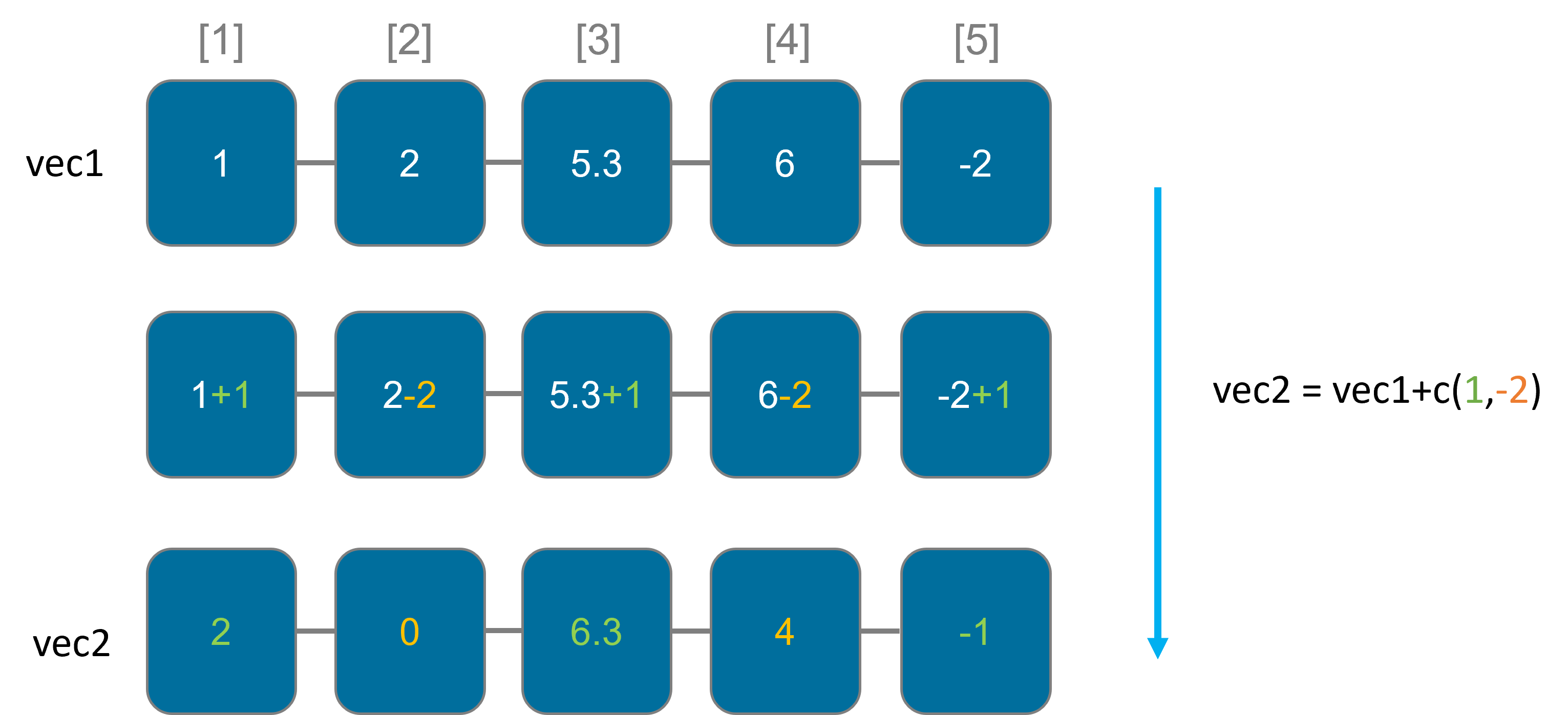
If you perform operations on vectors of different lengths, R will automatically recycle or repeat the shorter vector to match the length of the longer vector. This can be powerful but should be used with caution to avoid unexpected results.

Dataframe
A data frame is a two dimensional data structure. It is a special case of a list which has each component of equal length. Each column represents a variable, which must have the same data type, and each row represents an observation or a case. Unlike matrices, however, data frames can hold columns of different data types (e.g., numeric, character, factor, date, etc.). This tabular structure makes data frames suitable for storing and working with structured data and allows you to represent real-world datasets with mixed data types in a single data structure. Data frames are built with the data.frame() function
a <- c("A", "B", "C", "A", "B", "A", "A") # create a vector called a
b <- c("X", "X", "X", "X", "Y", "Y", "Y") # create a vector called b
c <- c(1, 2, 3, 4, 5, 6, 7) # create a vector called c
d <- c(10, 20, 30, 40, 50, 60, 70) # create a vector called d

# create a data frame from previous vectors with assigned column names to vectors.
df <- data.frame(Cat1 = a, Cat2 = b, Val1 = c, Val2 = d)

print(df)

   Cat1 Cat2 Val1 Val2
1    A    X    1   10
2    B    X    2   20
3    C    X    3   30
4    A    X    4   40
5    B    Y    5   50
6    A    Y    6   60
7    A    Y    7   70
Data frames have column names (variable names) and row names (often called row labels or row names) that help identify and reference specific variables and observations. You can access columns using the $ operator or square brackets [ ], and you can access rows by their index or labels. For more details, see Unit 04 You can use functions like str() to check the data type of the column. summary() summarizes the of the columns. For numeric variables, it provides basic summary statistics for that vector, including the minimum, 1st quartile, median, mean, 3rd quartile, and maximum values. Note, that you can also apply this function to vectors! If you want to quickly inspect the first few rows a long dataframe, you can use the head()-function. The default behavior of head() is to display the first 6 rows or elements, but you can specify a different number if needed.
With nrow() and ncol(), you can return the number of rows and columns, respectively.
str(df)
'data.frame':	7 obs. of  4 variables:
 $ Cat1: chr  "A" "B" "C" "A" ...
 $ Cat2: chr  "X" "X" "X" "X" ...
 $ Val1: num  1 2 3 4 5 6 7
 $ Val2: num  10 20 30 40 50 60 70

summary(df)
     Cat1               Cat2                Val1          Val2
 Length:7           Length:7           Min.   :1.0   Min.   :10
 Class :character   Class :character   1st Qu.:2.5   1st Qu.:25
 Mode  :character   Mode  :character   Median :4.0   Median :40
                                       Mean   :4.0   Mean   :40
                                       3rd Qu.:5.5   3rd Qu.:55
                                       Max.   :7.0   Max.   :70

head(df, n=3)
  Cat1 Cat2 Val1 Val2
1    A    X    1   10
2    B    X    2   20
3    C    X    3   30
Columns can be attached using cbind() or directly assigned:
BoolVec <- c(T,T,T,F,F,F,F)
df_vers2 <- cbind(df,BoolVec)
df_vers2
  Cat1 Cat2 Val1 Val2 BoolVec
1    A    X    1   10    TRUE
2    B    X    2   20    TRUE
3    C    X    3   30    TRUE
4    A    X    4   40   FALSE
5    B    Y    5   50   FALSE
6    A    Y    6   60   FALSE
7    A    Y    7   70   FALSE


df_vers3$BoolVec <- c(T,T,T,F,F,F,F)
df_vers2
  Cat1 Cat2 Val1 Val2 BoolVec
1    A    X    1   10    TRUE
2    B    X    2   20    TRUE
3    C    X    3   30    TRUE
4    A    X    4   40   FALSE
5    B    Y    5   50   FALSE
6    A    Y    6   60   FALSE
7    A    Y    7   70   FALSE
Matrix
A matrix is a two-dimensional rectangular data set. It can be created using a vector input to the matrix() function.
nrow stands for 2 rows and ncol for 3 columns. All data within a matrix must be of the same data type.
# Create a matrix.
M = matrix(c('a','a','b','c','b','a'), nrow = 2, ncol = 3)
print(M)
    [,1] [,2] [,3]
[1,] "a"  "b"  "b"
[2,] "a"  "c"  "a"
When we execute the above code, it produces the following result − Notice that by default, the first column is first filled from top to button, then the second column and so on.
it follows this pattern:

If you want to change this, set byrow=FALSE
M = matrix(c('a','a','b','c','b','a'), nrow = 2, ncol = 3, byrow = TRUE)
M
     [,1] [,2] [,3]
[1,] "a"  "a"  "b"
[2,] "c"  "b"  "a"
Columns and rows can be attached using cbind() and rbind(), respectively. With nrow() and ncol(), you can return the number of rows and columns, respectively. As in dataframes, you can add names to your columns and row. In contrast to dataframes, however, you cannot address a column with by ”$”.
Array
Arrays are the objects which can store data in more than two dimensions. For example − If we create an array of dimension (2, 3, 4) then it creates 4 rectangular matrices each with 2 rows and 3 columns. Arrays can store only one data type.
An array is created using the array() function. It takes vectors as input and uses the values in the dim parameter to create an array.
# create an array with numbers from 1 to 24 with the dimensions of 3 rows, 4 columns and 2 "tables".
my.array <- array(1:24, dim=c(3,4,2))

my.array
, , 1
   [,1] [,2] [,3] [,4]
[1,]  1  4  7  10
[2,]  2  5  8  11
[3,]  3  6  9  12
, , 2
   [,1] [,2] [,3] [,4]
[1,]  13  16  19  22
[2,]  14  17  20  23
[3,]  15  18  21  24
This array has three dimensions. Notice that, although the rows are given as the first dimension, the tables are filled column-wise. So, for arrays, R fills the columns, then the rows, and then the rest.
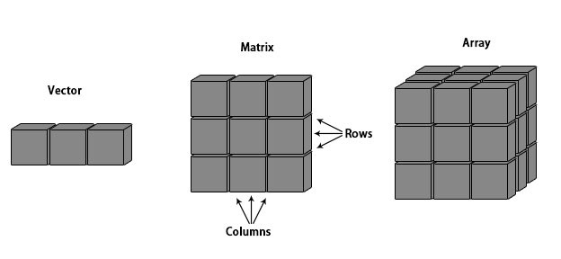
Visualized difference between vector, matrix and array:

A vector is one-dimensional, a matrix is two-dimensional and an array is more than two dimensional.
Lists
A list is an object which can contain many different types of elements inside it like vectors, a matrix, functions and even another list inside it.
The list is created using the list() function. Unlike matrices list elements do not need equal length and same data types.
# Create a list.
list1 <- list(c(2,5,3),21.3,sin)

# Print the list.
print(list1)
When we execute the above code, it produces the following result:
[[1]]
[1] 2 5 3

[[2]]
[1] 21.3

[[3]]
function (x)  .Primitive("sin")
It prints one list with three elements. The first element [[1]] is an vector containing values. The second element [[2]] is a value and the third [[3]] is a function. Note, that in lists, that the selection of list element via single square brackets [] preserves the list structure, which means that the result will still be a list if you extract a single element. while [[]] returns the actual value stored within the selected element. Therefore, the choice between [] and [[]] depends on whether you want to work with the structure of the list or extract the values from it.
list1[1]
[[1]]
[1] 2 5 3

list1[[1]]
[1] 2 5 3
As with our other non-atomic object type, the data frame, we can name the elements and address these elements with “$”
names(list1) <- c("numbers","my.double","my.sin")

list1$numbers
[1] 2 5 3
Factors
In R, a “factor” is a data structure used for fields that takes only predefined, finite number of values (categorical data). In such case, we know the possible values beforehand and these predefined, distinct values are called levels. Factors are more memory-efficient than storing categorical data as character vectors. This is because factors internally represent the data as integers and maintain a separate list of levels. They can have a specific order or hierarchy, which can be important when dealing with ordinal data. Factors with an order can be used in statistical analyses that consider the order of the levels. Using factors helps maintain data integrity by ensuring that values are limited to a predefined set of levels. This reduces the risk of errors and inconsistencies in data entry.
In such case, we know the possible values beforehand and these predefined, distinct values are called levels.
A factor is created using the function factor(). Levels of a factor are inferred from the data if not provided.
treecover <- factor(c("Spruce", "Spruce","Gap","Beech","Beech","Oak","Oak"))
treecover

[1] Spruce Spruce Gap Beech Beech Oak Oak
Levels: Beech Gap Oak Spruce
Here, we can see that factor treecover has seven elements and four levels. We can check if a object is a factor or not using class() function.
Similarly, levels of a factor can be checked using the levels() function.
class(treecover)
[1] "factor"

> levels(treecover)
[1] "Beech" "Gap" "Oak" "Spruce"
By default, the levels are assigned alphabetically. You can change this order by directly naming the levels in your preferred order while setting the factor:
treecover <- factor(c("Spruce", "Spruce","Gap","Beech","Beech","Oak","Oak"), levels=c("Gap","Spruce","Fir","Beech","Oak"))
treecover

[1] Spruce Spruce Gap Beech Beech Oak Oak
Levels: Gap Spruce Fir Beech Oak
When you define the factor levels explicitly, you are essentially specifying the allowed categories that this factor can have. This is a common practice, especially when you want to ensure that certain levels are present in the factor, or when you want to control the order of the levels. However, if you do not explicitly specify all the possible levels when creating a factor, R will, by default, assign missing values (NA) to any values that do not match the predefined levels. This behavior ensures that any values outside the defined levels are recognized as missing data.
treecover <- factor(c("Spruce", "Spruce","Gap","Beech","Beech","Oak","Oak","Birch"), levels=c("Gap","Spruce","Fir","Beech","Oak"))
treecover

[1] Spruce Spruce Gap Beech Beech Oak Oak <NA>
Levels: Gap Spruce Fir Beech Oak
If you are working with ordinal data, set ordered=T:
treecover <- factor(c("Spruce", "Spruce","Gap","Beech","Beech","Oak","Oak","Birch"), levels=c("Gap","Spruce","Fir","Beech","Oak"), ordered=T)
treecover

[1] Spruce Spruce Gap Beech Beech Oak Oak <NA>
Levels: Gap<Spruce<Fir<Beech<Oak
