
First Steps in R
Making your first steps in R with simple arithmetic operations.
#Hashtag and Run!
R treats the hashtag character, #, in a special way. It will not compile anything that follows a # on a line. This makes hashtags very useful for adding comments and annotations to your code. You will be able to read the comments, but your computer will pass over them.
# This is a comment. Comments are very helpful
# when you want to describe what's going on in your code.
# Use them often!
This is not a comment anymore. Be careful.

hello <- "Welcome to R" #the variable "hello" is storing the information "Welcome to R"
To run a chunk, you can hit the “Run” arrow to the right in the first Window (following picture, red box), or put your cursor inside the chunk and then hit CTRL + ENTER on Windows/Linux or CMD + ENTER on a Mac.
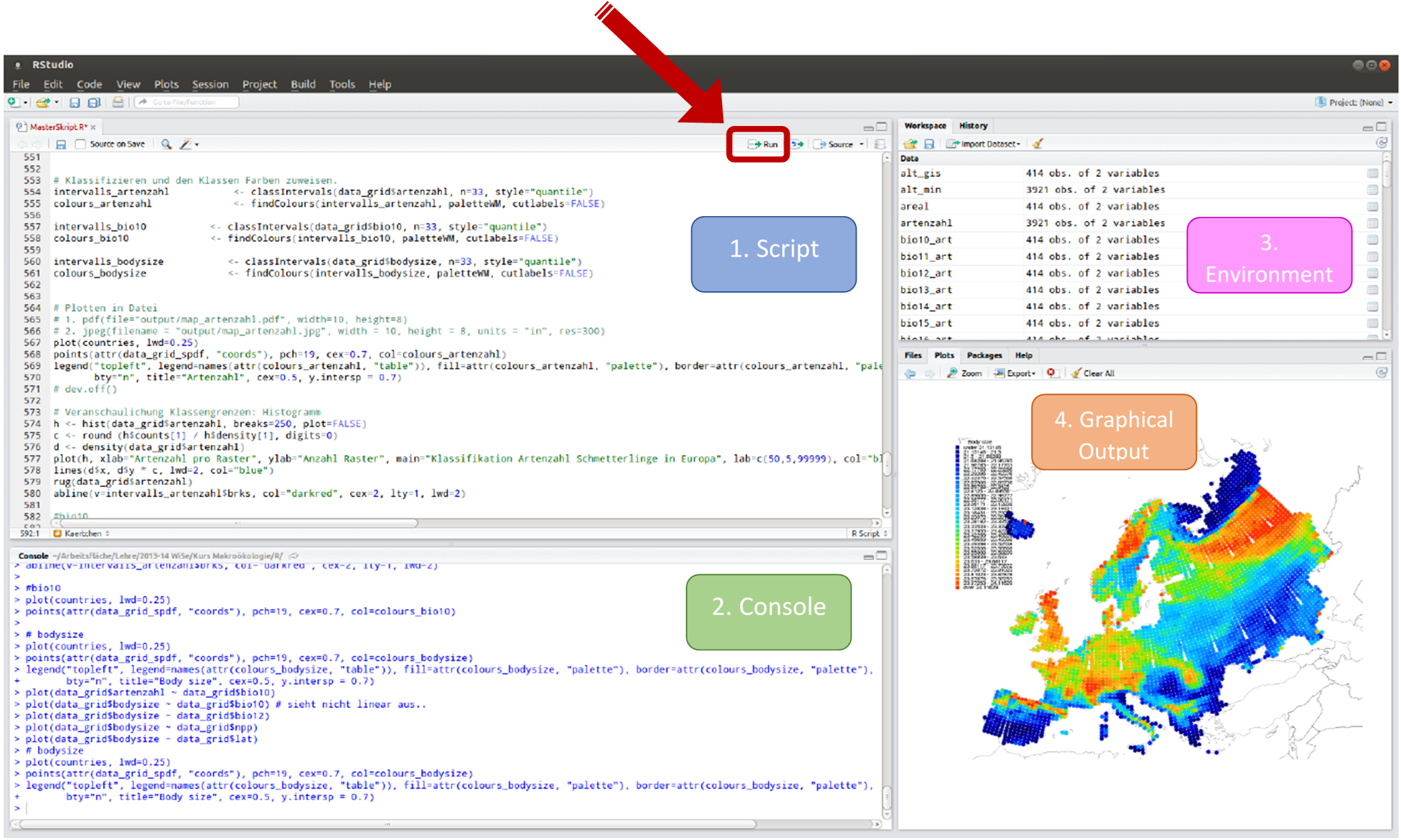
The code and the output of the code will print below the chunk in the second Window (Console). It looks like this:
> hello <- "Welcome to R"
> hello
[1] "Welcome to R"
>
Here, you’ll also see on the left hand side the “>” symbol which means that R is ready to receive a new command. If there’s a “+” is visible instead, this means that the command has not yet been completed, e.g. a parenthesis has not been closed.
Creating scalar objects and simple arithmetic operations
The basic arithmetic operations are addition, subtraction, multiplication and division. Further, more complex operations include square roots, exponentiation and some other. To control the order of operations, use parentheses “()”. Note, that square brackets “[]” cannot be used, because they are reserved for subsetting or indexing data structures like vectors, lists, data frames, and matrices, as you will see in Unit 04.
Examples of mathematic operations in R. This is using R like a calculator.
| Operator | Description | Example |
|---|---|---|
| Arithmetic Operators | ||
| + | Addition | x + y |
| - | Subtraction | x - y |
| * | Multiplication | x * y |
| / | Division | x / y |
| ^ or ** | Exponentiation | x^y |
| x %% y | Modulus (x mod y) | x %% y |
| %/% | Integer division | x %/% y |
| Math Functions | ||
| log() | Logarithms, by default natural | log(x) |
| exp() | Exponential function | exp(x) |
| sqrt() | Square-root | sqrt(x) |
| ^(1/n) | nth roots | x^(1/n) |
| abs() | Absolute value | abs(x) |
| sin() | Sine | sin(x) |
| cos() | Cosinus | cos(x) |
| tan() | Tangent | tan(x) |
This is what it looks like in R:
> 1 + 2
[1] 3
> 2 - 1
[1] 1
> 2 * 3
[1] 6
> 2 / 3
[1] 0,6666666666666667
> 2 ^ 3
[1] 8
> cos(2 ^ (3+2))
[1] 0.8342234
That [1] next to your result is a reminder that this line begins with the first value in your result. Some commands return more than one value, and their results may fill up multiple lines.
Assigning values to objects
And now you have reached the core concept of every object-based programming language: assigning objects. This fundamental operation is remarkably straightforward. You type in the name of the object-to-be, an assignment operator, and the content you’d like to assign. In R, there are two assignment operators: <- and =. The <- operator is the more common and recommended way to assign objects in R. It’s considered good practice because it makes your code more readable and is less likely to be confused with the equality operator ==, which is used for comparison.
> # Assign values to objects
> a <- 1+2 # addition/allocation, calculation is stored in object "a"
> a <- print the result
[1] 3
> # adding another object
> b <- 2-1
> b
[1] 1
>
> a + b # apply operators to objects
[1] 4
>
> c <- (a + b) * 2 # brackets
> c
[1] 8
And that is how information is stored in objects in an object-oriented programming language.