Time series clustering
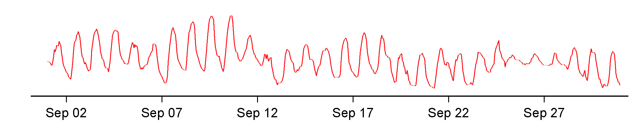
Just as one last example on time series analysis for this module and mainly for demonstrating that this module only tipped a very small set of analysis concepts out there, we will have a glimpse on time series clustering. To illustrate this concept, we will again use the (mean monthly) air temperature record of the weather station in Cölbe (which is closest to Marburg). The data has been supplied by the German Weather Service. For simplicity, we will remove the first six entries (July to December 2006 to have full years).
# read data we saved in unit 9
tam <- read.table("tam.txt", header = TRUE, sep = ";")
head(tam)
##     Date        Ta
## 1 200607 21.753970
## 2 200608 15.567473
## 3 200609 16.683194
## 4 200610 12.118817
## 5 200611  7.325556
## 6 200612  4.468011
# remove the first six entries for simplicity
tam <- tam[-(1:6),]
# convert Date column to POSIXlt Date; added day 01 for the conversion
tam$Date <- strptime(paste0(tam$Date, "01"), format = "%Y%m%d", tz = "CEST")
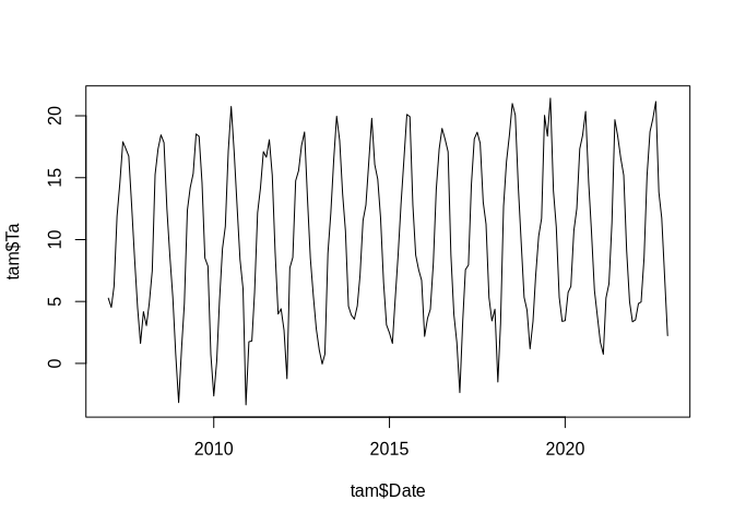
plot(tam$Date, tam$Ta, type = "l")
The major risk in time series clustering (or any other clustering) is that we cluster something, which actually does not have any kind of “real” groups. Hence, the most important part to remember is that cluster algorithms will always identify clusters no matter if they really exist. As a consequence: never use clustering if you are not sure that there definitively are groups in the data. Moreover, clustering is generally applied only if you have more than one time series from more than one location.
Of course there is no rule without exception and the one exception here is: if you want to show some code and do not want to introduce a new dataset just for this last example, you can use it on a dataset where you have no glimpse of a grouping as long as you are not the one who gets the grading in the end.
Aside from having no idea if we have a grouping and aside that we have only one single station record, let’s have a look at the above time series. There might be a difference between 2010 and the rest of the years since 2010 shows very warm summer and cold winter temperatures. To start with clustering, we will have to look at the individual years as different time series by transforming our data into a matrix with 12 columns (i.e. one for each month) and the required number of years. Thereby, we have to make sure that the original dataset is actually transformed into the matrix format by rows and not by columns. This will result in a matrix with one year per row:
tam_ta <- matrix(tam$Ta, ncol = 12, byrow = TRUE)
row.names(tam_ta) <- paste0(seq(2007, 2022))
tam_ta
##           [,1]        [,2]      [,3]      [,4]     [,5]     [,6]     [,7]
## 2007  5.268683  4.53095238 6.2369624 11.882361 14.57567 17.89889 17.34704
## 2008  4.178226  3.05474138 4.8426075  7.477222 15.24677 17.32917 18.45255
## 2009 -3.158871  1.30922619 4.8364247 12.364861 14.19651 15.32306 18.52773
## 2010 -2.627823  0.20758929 5.0146505  9.270000 11.06237 17.16667 20.75013
## 2011  1.752285  1.81413690 5.7346774 12.165139 14.15618 17.10208 16.65296
## 2012  2.683468 -1.23189655 7.7043011  8.555278 14.74812 15.57597 17.59153
## 2013  1.092070 -0.04494048 0.7533602  8.902222 12.11250 16.44056 19.96048
## 2014  3.575000  4.64568452 7.0896505 11.548194 12.78562 16.32681 19.79220
## 2015  2.461022  1.62306548 5.0916667  8.785694 12.88306 16.49889 20.10591
## 2016  2.184677  3.64382184 4.3685484  8.124861 14.03199 17.31597 18.97796
## 2017 -2.356048  3.43883929 7.5743280  7.946806 14.41142 18.13806 18.67043
## 2018  4.378898 -1.49925595 3.2267473 12.705278 16.28723 18.45139 20.98952
## 2019  1.182258  3.38601190 7.0571237 10.277222 11.70659 20.03375 18.35600
## 2020  3.457124  5.73821839 6.2223118 10.730972 12.50188 17.32931 18.42016
## 2021  1.723790  0.74404762 5.2905914  6.442500 11.34368 19.68181 18.34825
## 2022  3.516935  4.83750000 4.9598118  8.570139 15.15296 18.71167 19.75430
##          [,8]     [,9]     [,10]    [,11]      [,12]
## 2007 16.73898 12.67542  8.470296 4.480000  1.6173387
## 2008 17.82917 12.47181  8.755780 5.336667  0.7397849
## 2009 18.33374 14.57264  8.515054 7.857917  0.7282258
## 2010 16.98454 12.57486  8.378898 6.022083 -3.3438172
## 2011 18.06210 15.17806  8.975538 3.989167  4.4114247
## 2012 18.68952 13.27528  8.509005 5.440694  2.8017473
## 2013 18.01801 13.68875 10.692608 4.619167  3.9010753
## 2014 16.05228 14.87569 11.748790 6.533889  3.1159946
## 2015 19.93105 12.79472  8.746774 7.553333  6.7141129
## 2016 18.11089 17.09653  8.751210 3.957778  1.7149194
## 2017 17.78078 13.03278 11.249462 5.314444  3.4383065
## 2018 20.04140 14.25931  9.822715 5.335694  4.2998656
## 2019 21.41890 13.94278 11.014516 5.338472  3.3940860
## 2020 20.34772 14.67410 10.608871 5.903194  3.8330645
## 2021 16.58638 15.19500  9.152016 4.992083  3.3623656
## 2022 21.14745 13.83819 11.725672 6.912083  2.2442204
This matrix can subsequently be used to compute the dissimilarity between the individual time series. In this example, we use the TSclust::diss function with method “DTWARP” (which is one of many, each leading to a different result; p gives the decaying of the auto-correlation coefficient to be considered).
tam_dist <- TSclust::diss(tam_ta, "DTWARP", p = 0.05)
tam_dist
##          2007     2008     2009     2010     2011     2012     2013     2014
## 2008 19.24069
## 2009 30.79566 31.27686
## 2010 41.22420 39.78805 38.00132
## 2011 22.79959 30.53591 27.06892 42.14468
## 2012 29.35046 21.24988 36.84308 41.79336 31.11600
## 2013 40.45138 40.87593 41.37245 35.56177 25.98853 29.09403
## 2014 26.78914 33.90738 36.86756 40.04724 28.75914 36.35242 32.43355
## 2015 35.82190 30.72825 33.32398 32.51645 28.84693 29.41835 28.72208 29.13347
## 2016 23.15795 19.50518 31.47002 43.05289 20.96015 25.73721 32.33223 30.89450
## 2017 30.75250 22.67033 38.39494 40.17789 35.51358 22.23133 30.30811 33.04461
## 2018 38.37680 35.55872 38.23498 46.21456 27.87125 34.87994 29.27271 30.92867
## 2019 37.62395 36.81298 43.30056 43.74769 35.43320 37.05981 22.81779 25.41953
## 2020 29.46244 31.18338 37.89050 39.45226 21.07195 35.50115 31.88983 19.38225
## 2021 28.20694 34.94268 33.28278 37.40041 19.27723 37.61231 28.43564 26.24180
## 2022 33.33505 24.19531 35.10020 42.44488 39.88704 28.67564 41.08707 24.16946
##          2015     2016     2017     2018     2019     2020     2021
## 2008
## 2009
## 2010
## 2011
## 2012
## 2013
## 2014
## 2015
## 2016 32.72350
## 2017 38.81933 25.53853
## 2018 32.86640 37.02209 36.24021
## 2019 36.00403 36.63025 24.27164 30.63571
## 2020 28.86440 30.54257 31.01781 23.97460 20.27760
## 2021 34.07328 28.80359 34.94257 36.95792 22.82116 25.03672
## 2022 26.30120 32.35828 28.57497 35.20857 28.75007 27.37277 40.29093
The resulting dissimilarity is larger if the different time series (i.e. years in this case) are less similar and smaller if they are more similar. This dissimilarity is now used for hierarchical clustering, which computes the distance between the individual samples. Plotting the result shows a cluster dendrogram:
tam_hc <- hclust(tam_dist)
plot(tam_hc)
rect.hclust(tam_hc, k = 3)
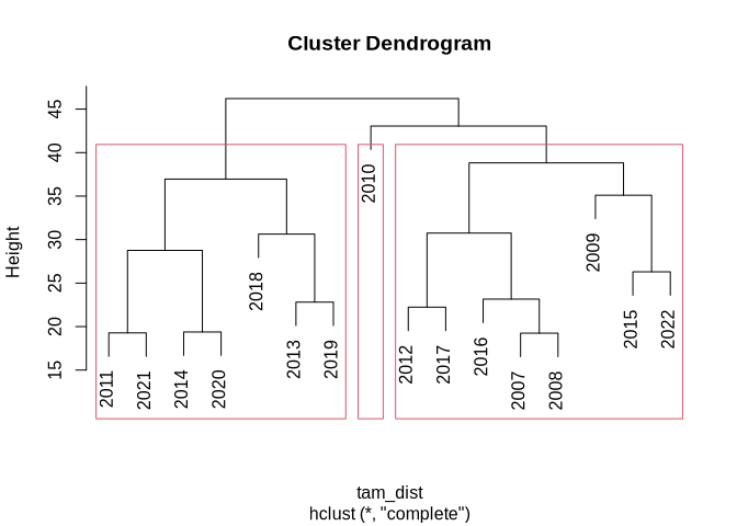
In this example, we derived three clusters of years with similar mean monthly air temperatures. The year 2010 forms a group on its own at the root of the dendrogram.
cutree(tam_hc, k = 3)
## 2007 2008 2009 2010 2011 2012 2013 2014 2015 2016 2017 2018 2019 2020 2021 2022
##    1    1    1    2    3    1    3    3    1    1    1    3    3    3    3    1