Time Series Decomposition
After looking into time-series forecasting, we will now switch to some basics of describing time series. To illustrate this, we will again use the (mean monthly) air temperature record of the weather station in Cölbe (which is closest to Marburg). The data has been supplied by the German Weather Service. For simplicity, we will remove the first six entries (July to December 2006 to have full years).
# read data we saved in unit 9
tam <- read.table("tam.txt", header = TRUE, sep = ";")
head(tam)
##     Date        Ta
## 1 200607 21.753970
## 2 200608 15.567473
## 3 200609 16.683194
## 4 200610 12.118817
## 5 200611  7.325556
## 6 200612  4.468011
# remove the first six entries for simplicity
tam <- tam[-(1:6),]

# convert Date column to POSIXlt Date; added day 01 for the conversion
tam$Date <- strptime(paste0(tam$Date, "01"), format = "%Y%m%d", tz = "CEST")

plot(tam$Date, tam$Ta, type = "l")
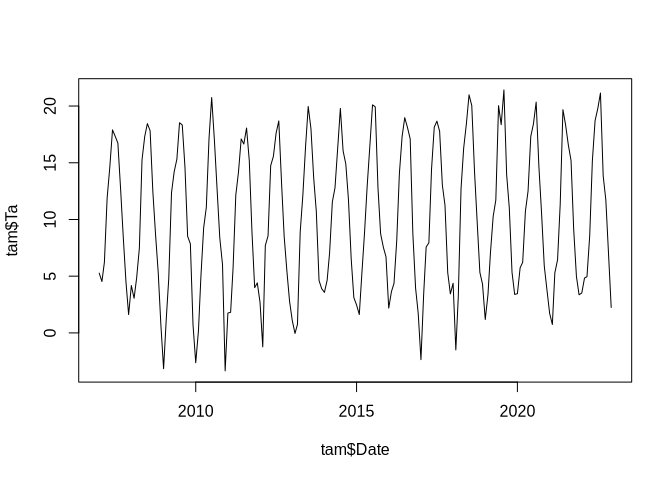
Seasonality of time series
The time series shows clear seasonality. In this case, we already know that monthly mid-latitude temperature shows a seasonality of 12 months.
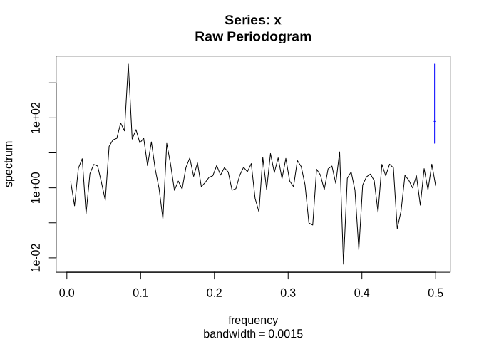
In case we are not certain, we could also have a look at the spectrum using e.g. the spectrum functions, which estimate the (seasonal) frequencies of a data set using an auto-regressive model.
The smallest frequency which is checked is 1 divided by the length of the time series. Hence, in order to convert frequency back to the original time units, we divide 1 by the frequency:
spec <- spectrum(tam$Ta)
plot(1/spec$freq, spec$spec, type = "h")
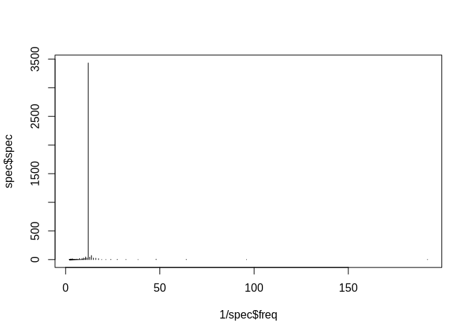
1/spec$freq[spec$spec == max(spec$spec)]
## [1] 12
The frequency of 12 months dominates the spectral density.
Decomposition of time series
Once we are certain about the seasonal frequency, we can start with the decomposition of the time series, which is assumed to be the sum of
- an annual trend,
- a seasonal component, and
- a non-correlated reminder component (i.e. white noise).
To start with the annual component or “trend”, we could use a 12 months running mean filter.
In the following example, we will use the rollapply function for that:
annual_trend <- zoo::rollapply(tam$Ta, 12, mean, align = "center", fill = NA)
plot(tam$Date, tam$Ta, type = "l")
lines(tam$Date, annual_trend, col = "red")
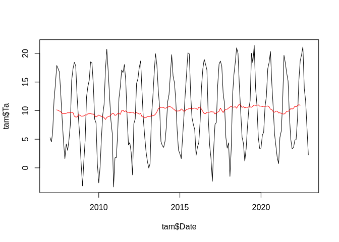
The annual trend shows some fluctuations but it is certainly not very strong or even hardly different from zero.
Once this trend is identified, we can subtract it from the original time series in order to get a de-trended seasonal signal, which will be averaged in the second step. The average of each will finally form the seasonal signal:
seasonal <- tam$Ta - annual_trend
seasonal_mean <- aggregate(seasonal, by = list(rep(seq(1,12), 18)),
                           FUN = mean, na.rm = TRUE)
plot(tam$Date, seasonal, type = "l")
lines(tam$Date, rep(seasonal_mean$x, 16), col = "blue")
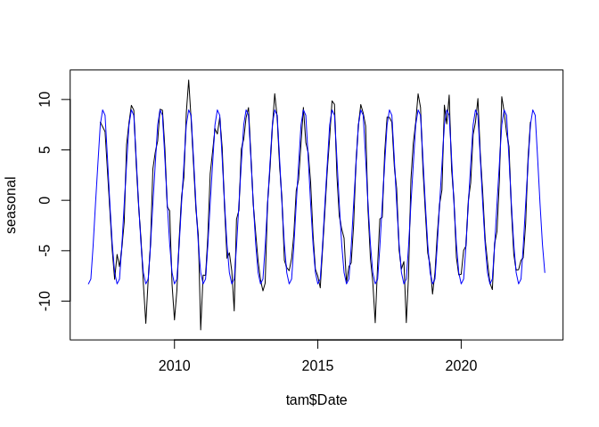
The blue line shows the average seasonal signal of the time series.
The only thing remaining is the remainder, i.e. the component not explained by neither the trend nor the seasonal signal:
remainder <- tam$Ta - annual_trend - seasonal_mean$x
plot(tam$Date, remainder, type = "l")
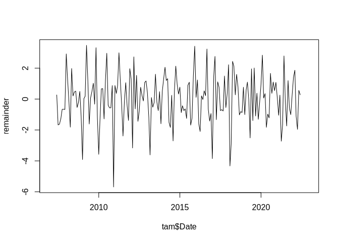
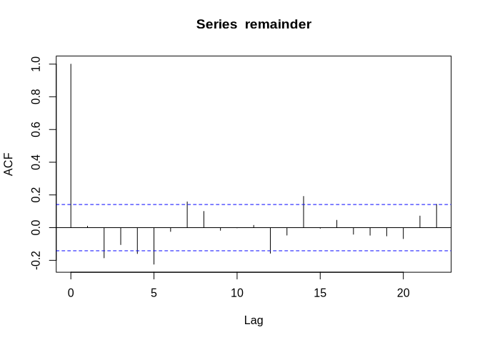
As we can see, it is slightly autocorrelated:
acf(remainder, na.action = na.pass)
As an alternative to the workflow above, we could (and should) of course use existing functions, like decompose, which handles the decomposition in one step.
Since this function requires a time series, this data type has to be created first.
Note that the frequency argument in the time series function does not correspond to the seasonal component but to the number of sub-observations within each major time step (i.e. monthly values within annual major time steps in our case):
tam_ts <- ts(tam$Ta, start = c(2007, 1), end = c(2022, 12), frequency = 12)
tam_ts_dec <- decompose(tam_ts)
plot(tam_ts_dec$trend)
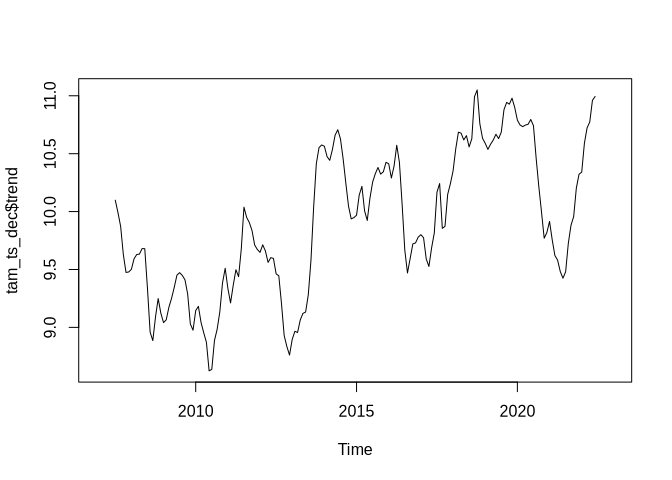
While the above shows the plotting of the trend component, we can also plot everything in one plot:
plot(tam_ts_dec)
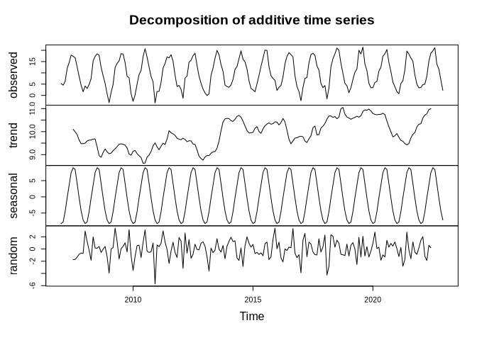
But - again - it is not as static as it seems.
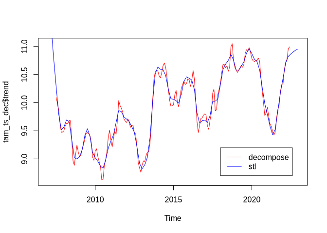
While decompose computes the (annual/long-term) trend using a moving average, the stl function uses a loess smoother.
Here is one realization using “periodic” as the smoothing window, for which - according to the function description - “smoothing is effectively replaced by taking the mean”.
The visualization shows the different long-term trends retrieved by the two approaches:
tam_ts_stl <- stl(tam_ts, "periodic")
plot(tam_ts_dec$trend, col = "red")
lines(tam_ts_stl$time.series[, 2], col = "blue")
legend(2018, 9.2, c("decompose", "stl"), col = c("red", "blue"), lty=c(1,1))
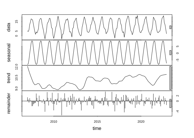
The entire result from the stl function call looks like this:
plot(tam_ts_stl)
Trend estimation
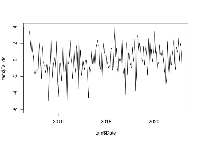
While the above helps us decompose a time series into several components, we are sometimes also interested in linear trends over time. Since seasonal signals strongly influence such trends, we generally remove the seasonal signal and analyze the anomalies. In order to remove the seasonal signal, we can average over all values for each month and subtract it from the original time series:
monthly_mean <- aggregate(tam$Ta, by = list(substr(tam$Date, 6, 7)), FUN = mean)
tam$Ta_ds <- tam$Ta - monthly_mean$x
plot(tam$Date, tam$Ta_ds, type = "l")
Once this is done, a linear model could be used. In this context, it is important to understand the meaning of the independent (i.e. time) variable. The following shows the slope of the trend per month since the time is just supplied as a sequence of natural numbers:
lmod <- lm(tam$Ta_ds ~ seq(nrow(tam)))
summary(lmod)
##
## Call:
## lm(formula = tam$Ta_ds ~ seq(nrow(tam)))
##
## Residuals:
##     Min      1Q  Median      3Q     Max
## -5.7249 -1.0009 -0.0431  1.1033  4.0367
##
## Coefficients:
##                 Estimate Std. Error t value Pr(>|t|)
## (Intercept)    -0.606272   0.238536  -2.542  0.01183 *
## seq(nrow(tam))  0.006283   0.002143   2.931  0.00379 **
## ---
## Signif. codes:  0 '***' 0.001 '**' 0.01 '*' 0.05 '.' 0.1 ' ' 1
##
## Residual standard error: 1.646 on 190 degrees of freedom
## Multiple R-squared:  0.04326,    Adjusted R-squared:  0.03822
## F-statistic: 8.591 on 1 and 190 DF,  p-value: 0.003793
If we were interested in annual trends, we could multiply the above slope of the time variable by 12 or define the time variable in such a way that each month is counted as a fraction of 1 (e.g. January 2006 = 2006; February 2006 = 2006.0084 etc.):
ts <- seq(from = 2007, to = 2024 + 11/12, by = 1/12)
lmod <- lm(tam$Ta_ds ~ ts)
summary(lmod)
##
## Call:
## lm(formula = tam$Ta_ds ~ ts)
##
## Residuals:
##     Min      1Q  Median      3Q     Max
## -5.7249 -1.0009 -0.0431  1.1033  4.0367
##
## Coefficients:
##               Estimate Std. Error t value Pr(>|t|)
## (Intercept) -151.91048   51.82860  -2.931  0.00379 **
## ts             0.07539    0.02572   2.931  0.00379 **
## ---
## Signif. codes:  0 '***' 0.001 '**' 0.01 '*' 0.05 '.' 0.1 ' ' 1
##
## Residual standard error: 1.646 on 190 degrees of freedom
## Multiple R-squared:  0.04326,    Adjusted R-squared:  0.03822
## F-statistic: 8.591 on 1 and 190 DF,  p-value: 0.003793
plot(ts, tam$Ta_ds, type = "l")
abline(lmod, col = "red")
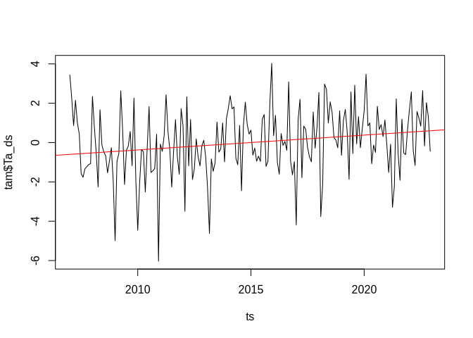
There is a significant annual trend.