Example: Workflow in R
This example provides a schematic workflow for processing vector and raster data in R.
Get raster data
Firstly, we import some raster data into our working environment
Therefore, we need to load a package to handle raster data in R, preferable terra. To get some example data we will use the package geodata
If the packages are not available, we need to install it first with install.packages("terra").
library(terra)
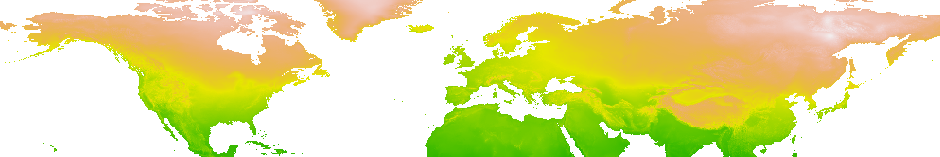
We now can use the function getData() to download some raster data: In this example a global map of precipitation values at 10 minutes spatial resolution.Set a path to a temporary folder where you want to store the downloaded data.
prec <- geodata::worldclim_global(var="prec", res=10, path="D:/temp")
Fortunately, the downloaded data already have a correct CRS:
##class       : SpatRaster
##dimensions  : 1080, 2160, 12  (nrow, ncol, nlyr)
##resolution  : 0.1666667, 0.1666667  (x, y)
##extent      : -180, 180, -90, 90  (xmin, xmax, ymin, ymax)
##coord. ref. : lon/lat WGS 84 (EPSG:4326)
##sources     : wc2.1_10m_prec_01.tif
##              wc2.1_10m_prec_02.tif
##              wc2.1_10m_prec_03.tif
##              ... and 9 more source(s)
##names       : wc2.1~ec_01, wc2.1~ec_02, wc2.1~ec_03, wc2.1~ec_04, wc2.1~ec_05, wc2.1~ec_06, ...
##min values  :           0,           0,           0,           0,           0,           0, ...
##max values  :         908,         793,         720,        1004,        2068,        2210, ...
… and can be quickly and simply visualized with terra::plot().
Note that the object type is a SpatRaster with 12 layers, one for each month of the year.
terra::plot(prec$wc2.1_10m_prec_01)
Get vector data
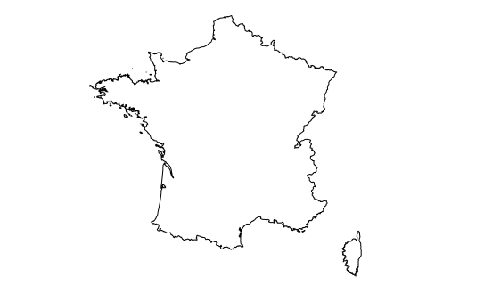
Secondly, we add some vector data to our working environment. For example the administrative boundaries of France at the country level:
fra <- geodata::gadm(country='FRA', level=0, path="D:/temp")
Fortunately, also these downloaded data already have a CRS:
## class       : SpatVector
## geometry    : polygons
## dimensions  : 1, 2  (geometries, attributes)
## extent      : -5.143751, 9.560416, 41.33375, 51.0894  (xmin, xmax, ymin, ymax)
## coord. ref. : lon/lat WGS 84 (EPSG:4326)
## names       : GID_0 COUNTRY
## type        : <chr>   <chr>
## values      :   FRA  France
Note that the object type here is a SpatVector (defined in package terra) with one feature (i.e. with a single polygon),
a certain extent (which can also be extracted with terra::ext(fra)), a CRS (which can be extracted with terra::crs(fra)), and two variables with some values (in this case country abbreviation and name).
Also vector data can quickly and simply be visualized with plot()
plot(fra)
Set extent
We can use the extent of one spatial object to crop (i.e. to cut out) another spatial object.
In this example, we will crop the raster map(s) with the extent defined in the vector object.
This is going to work because both objects have the same CRS.
Note that crop() processes all layers of the input raster stack.
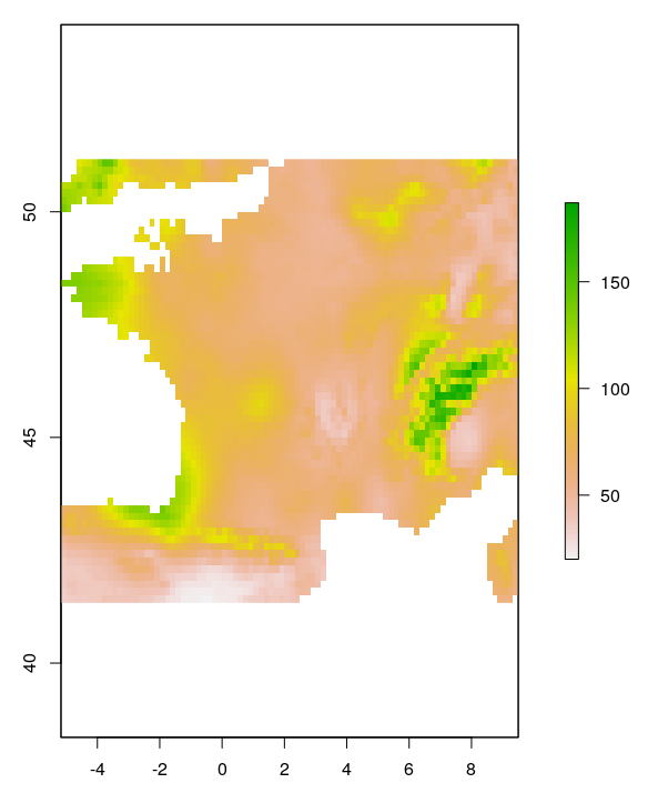
cropped_prec <- crop(prec, ext(fra))
For function arguments see ?crop(). Now we have precipitation maps of France:
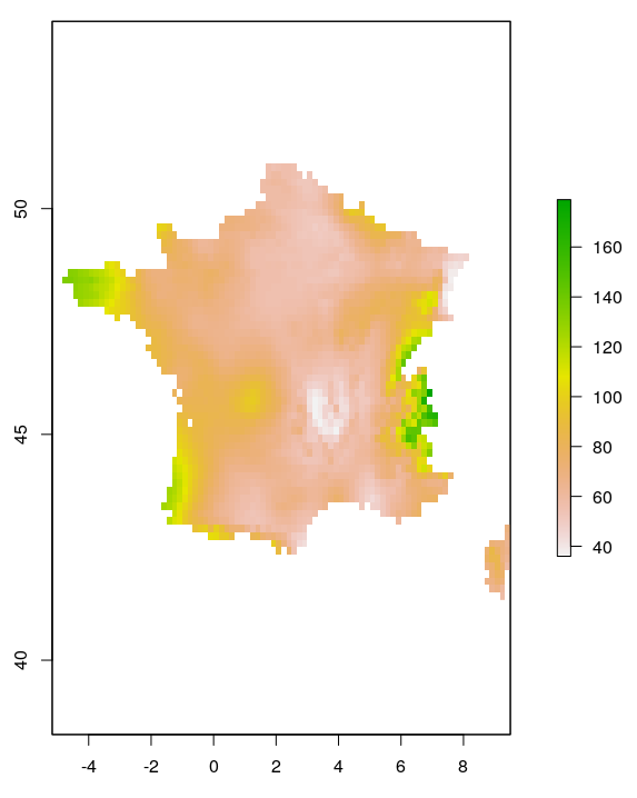
plot(cropped_prec$wc2.1_10m_prec_01)
Vector operations
A simple vector operation would be to clip a spatial object not by the extent of another spatial object but by features or polygons of any shape.
We will now use the country boundary of France for clipping of the already cropped precipitation maps with the mask() function of the raster package:
clipped_prec <- mask(cropped_prec, fra)
The result is a SpatRaster object with 12 layers, one for each month of the year.
Again, the result can quickly and simply be visualized with plot()
plot(clipped_prec$wc2.1_10m_prec_01)
Raster operations
The created SpatRaster now contains precipitation values of France on a monthly basis. What if we want to have a single precipitation layer with annual precipitation values? We would need to sum up the values of all 12 precipitation layers for each pixel location. This can be done by:
clipped_prec_sum <- sum(clipped_prec)
The resulting raster map looks like this:
plot(clipped_prec_sum)
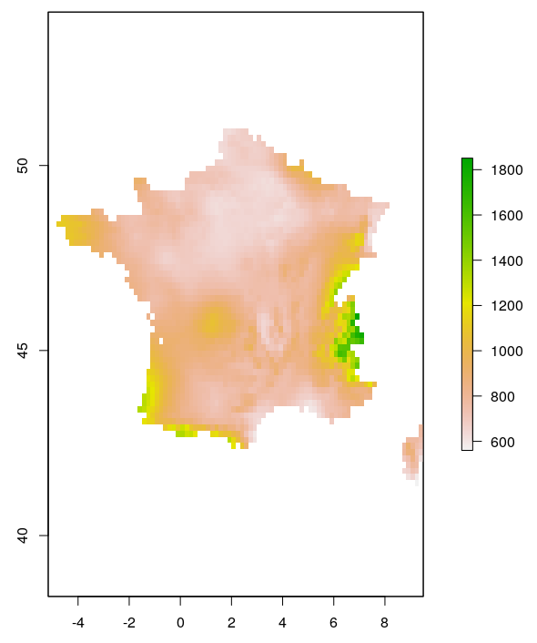
Note the different value range, which now stands for the annual amount of precipitation (in mm).
Mapping
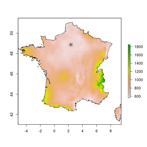
We now combine all the above created spatial objects to create a single simple map:
plot(clipped_prec_sum)
plot(fra, add=T)
points(2.349014, 48.864716, pch=8, cex=2) # roughly the location of Paris
Write out
The above created overlay of maps can be written to file as an ordinary image with e.g.
jpeg("FirstSimpleMap.jpg")
plot(clipped_prec_sum)
plot(fra, add=T)
points(2.349014, 48.864716, pch=8, cex=2)
dev.off()
Note that this is a raster image without geographic information.
If you want to write out the spatial objects with geographic information, use e.g. terra::writeRaster() or raster::writeVector().
Other important functions
- Reading in raster data from file:
terra::rast() - Reading in vector data from file:
terra::vect()
More information
For more details see www.rspatial.org and Geocomputation with R
Comments?
You can leave comments under this issue if you have questions or comments about the content on this page. Please copy the corresponding line into your comment to make it easier to answer the question.