LM Presence-only SDM model evaluation

In the last exercise, we calculated some evaluation metrics for the model we created for Aglais caschmirensis in Pakistan. Since we only had presence-only test points, we had to generate background points to calculate evaluation metrics that are based on binary data.

We use these metrics to assess how good a model or a map is. However, we usually have no information on the “goodness” of the evaluation metrics themselves. Today, we will look at how reliable the metrics we use to assess models actually are.

There are several components that could potentially influence the reliability of these metrics:

• The use of background points: It is known that these introduce bias, but how much exactly?
• Sample size: How many presence points do I actually need for a reliable evaluation?
• Number of background points: How many background points are required to calculate these metrics accurately?
• Sampling methods: Is there a better way to sample points compared to standard random background points?

Sample size

After splitting your test dataset from the training data, you probably had around 10 test points for evaluation. While it has been suggested that modeling species distributions with as few as 3 presence points is possible, this depends heavily on the species’ niche width (van Proosdij et al. 2025). The calculation of evaluation metrics likely requires more points than the modeling process itself to obtain reliable results. Some studies suggest a minimum of 30 points for stable evaluation, though further research on this topic is needed ( Jiménez-Valverde 2020).

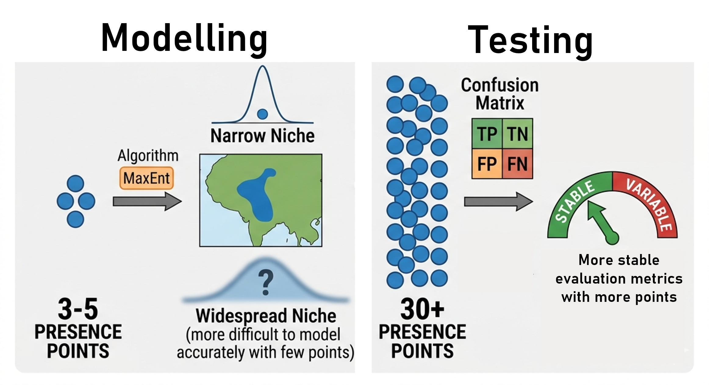
Figure: Number of points needed for modelling and testing. Generated with Google Gemini, edited.

Number of background points.

Many studies use the same number of background points for calculating evalaution metrics as they also use for modeling. However this leads to imbalanced datasets on which the evaluation metrics are calculated which is in general not recommened (Lobo et al., 2006).

The figure below illustrates the agreement between actual model performance and the calculated evaluation metrics. If a metric estimates the model performance perfectly, all points would align exactly on the red diagonal line.

• Balanced Dataset (Top): The upper panel shows models where evaluation metrics were calculated using a balanced dataset.

• Imbalanced Dataset (Bottom): The lower panel displays metrics calculated on an imbalanced dataset.

As you can observe, imbalance leads to a significantly higher error rate in the evaluation metrics (an increase in Mean Absolute Error, or MAE), which results in a distorted assessment of the model’s true quality.

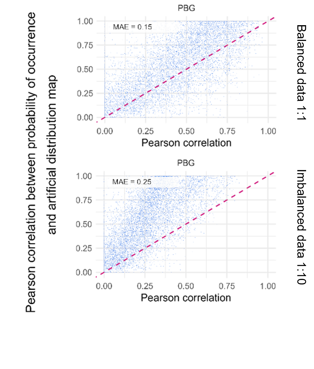
Figure: Performance of evaluation metric Pearson’s correlation on balanced and imbalanced test data. In each plot, one evaluation metric with rescaled values from 0 to 1 is shown on the x-axis, and Pearson’s correlation between the true probability of occurrence and the artificial distribution maps (used as the reference for actual model performance) is shown on the y-axis. The dotted pink line depicts the bisector (slope = 1, intercept = 0). Each blue point represents one evaluation metric calculated on one of the 8,335 experimental test datasets. Median absolute error (MAE) in the upper left corner of each plot. Bald et al. (under review)

Sampling methods

Most studies rely on random background points to evaluate the models. These points are however just randomly distributed over the study area. This means that depending on your niche width you are more likely to get higher or lower evaluation metrics. For example, if your niche is very small and your background points are distributed randomly over the study area, they are more likely to be sampled in areas where the species is absent, leading to inflated evaluation metrics. If the niche of your species is very broad you are more likely to sample in suitable areas creating a worse evaluation result.

An alternative to this approach is to sample background points via the environmental space by sampling points in areas that are environmentaly distant from the presence points. These points are either called pseudo-absences or artificial-absence data sometimes also invented-absence data. We can achieve somewhat lower errors in the evaluation metrics by distant environmental space for artificial-absences as you can see in the figure below.

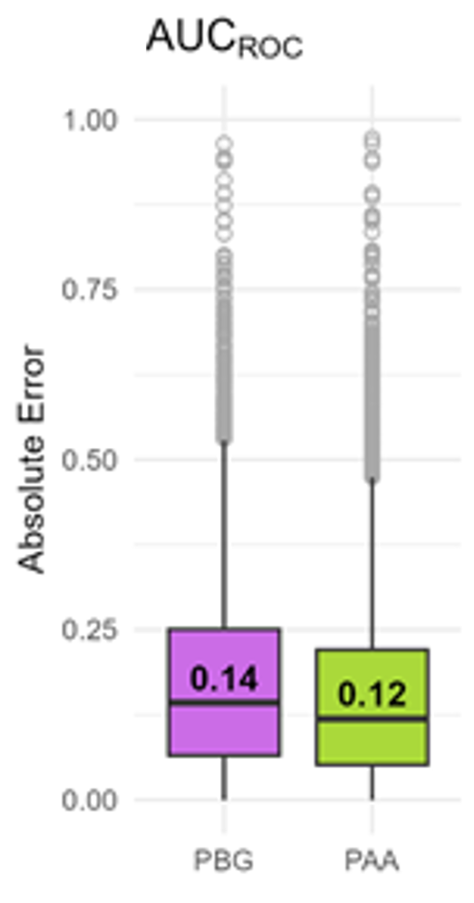
Figure: Absolute errors of evaluation metrics. Comparison of absolute errors calculated on presence-background (PBG; purple), and presence-artificial-absence (PAA; green). Each box plot is based on 8,335 data points. Outliers in gray. Low absolute error indicates good assessment of the artificial distribution maps by the evaluation metric. Median absolute error is indicated in the boxplot. Bald et al. (under review)