LM Model evaluation

Model evaluation is the process of assessing how good or reliable a model as well as its predictions are. Also we want to determine the model’s ability to generalize. A model that performs perfectly on its training data but fails to predict independent observations is overfitted, meaning it has memorized the training data by heart but it is not able to make valuable assumptions about data that deviates from the training data. Ideally effective evaluation would allows us to communicate the quality of our models to stakeholders and researchers and ensure that conservation decisions are based on robust evidence.

Figure: Noisy (roughly linear) data is fitted to a linear function and a polynomial function. Although the polynomial function is a perfect fit, the linear function can be expected to generalize better: If the two functions were used to extrapolate beyond the fitted data, the linear function should make better predictions. Source: Wikimedia, Author: ThirdOrderLogic, CC BY 4.0

However, in Species Distribution Modeling the model assessment is especially difficult and Leroy (2022) listed evaluation metrics as one of the unresolved fields in SDM. Why is that? To fully understand this issue we will first have a look at how evaluation metrics are calculated in SDM and in machine learning in general.

Figure: Choosing presence-only species distribution models. Source: Boris Leroy 2022, https://doi.org/10.1111/jbi.14505.

Evaluation metrics in SDM

In Species Distribution Modeling a lot of the metrics are standard machine learning evaluation metrics. Here we differentiate between threshold-dependent and threshold-independent metrics.

Threshold-Dependent Metrics

When your study design includes presence-absences (binary data [0,1]) you can utilize the standard machine learning Confusion Matrix. This matrix serves as the foundation for most classification statistics by categorizing outcomes into True Positives, True Negatives, False Positives, and False Negatives.

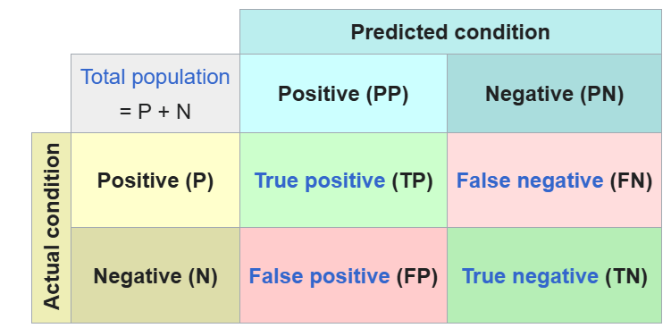
Figure: Confusion matrix. Source: Wikipedia

Commonly used evaluation metrics include:

Accuracy: This is the most intuitive metric, representing the overall proportion of correct predictions (both Presences and Absences).
- Calculation: (TP + TN) / (TP + TN + FP + FN)
- Critical Note: Accuracy is often misleading in SDM due to “Prevalence Bias.” If a species is rare (e.g., present in only 1% of the landscape), a model can achieve 99% accuracy simply by predicting the species is absent everywhere, failing to capture the actual niche entirely.
Sensitivity (True Positive Rate): Measures the model’s ability to correctly identify occupied sites. A model with low sensitivity suffers from “Omission errors” (missing the species where it actually is).
- Calculation: TP / (TP + FN)
Specificity (True Negative Rate): Measures the ability to correctly identify unoccupied sites. A model with low specificity suffers from “Commission errors” (predicting the species where it is not).
- Calculation: TN / (TN + FP)
Cohen’s Kappa: Measures the agreement between the model and the observations, corrected for the agreement that might occur by chance.
- Calculation: (Observed Accuracy - Expected Accuracy) / (1 - Expected Accuracy)
  - Where Observed Accuracy = (TP + TN) / Total
  - Where Expected Accuracy = [((TP + FN) * (TP + FP)) + ((FP + TN) * (FN + TN))] / (Total * Total)

For a comprehensive overview of the evaluation metrics, you may refer to the study by Konowalik & Nosol (2021), which provides an extensive analysis of over 30 different evaluation metrics used in SDM.

While many of these metrics originate from general ecological context, others have been specifically proposed for SDM. A primary example is the True Skill Statistic (TSS). The TSS was introduced as an advancement over Cohen’s Kappa to address the latter’s problematic sensitivity to species prevalence.

In ecological studies, TSS is often preferred because it provides a measure of performance that is more independent of the species’ prevalence (the frequency of occurrence in the dataset). It is calculated as the sum of sensitivity and specificity minus one (Sensitivity + Specificity - 1). The resulting values range from -1 to +1. In modeling practice, TSS values above 0.6 are generally considered to indicate high model utility, while a value of 0 suggests the model performs no better than random. The theoretical foundation for the superiority of this metric over Kappa can be found in the work of Allouche et al. (2006).

Note: Look at the classes in the confusion matrix, what do you notice about the data type. Also think about the data you have set aside for model testing and the maps that you have produced. What potential challenges do you anticipate?

Threshold-Independent Metrics

Next to metrics calculated on a confusion matrix and therfore in need of an threshold there are also threshold-independent metrics available.

The most ubiquitous metric in SDM is the Area Under the Receiver Operating Characteristic curve (AUC-ROC). The advantage of AUC is that it evaluates the model across all possible thresholds simultaneously. It effectively represents the probability that the model will rank a randomly chosen presence site higher than a randomly chosen absence site. An AUC of 0.5 suggests the model is performing no better than a random guess, while an AUC of 1.0 represents perfect discrimination.

Although the Area Under the Receiver Operating Characteristic Curve (AUC) remains the most frequently utilized evaluation metric in Species Distribution Modeling and is the default evaluation metric in the widely used Maxent software, it has also been subject to significant critique. There are complete studies available that focus primarily on why AUC should not be used for SDM assessment, for example, “AUC: a misleading measure of the performance of predictive distribution models“ (Lobo et al., 2008).

Critics argue that AUC can be artificially inflated by the geographic extent of the study area, as including large regions far from the species’ known range makes it easier for the model to distinguish presence from absence without necessarily capturing fine-scale ecological requirements.

Evaluation metrics and SDM: Challenges

To calculate evaluation metrics, two distinct data types must be available: first, the predicted distribution map generated by your model, and second, the ground truth or test data used as a reference. In the context of Species Distribution Modeling, both of these data components introduce unique challenges that can complicate the assessment of model performance:

Species distribution maps

The primary challenge with SDM outputs is that most algorithms, such as Generalized Linear Models (GLM), Maxent, or Random Forests, do not produce a map of “Presence” and “Absence.” Instead, they yield a continuous surface of suitability or probability ranging from 0 to 1.

To use the majority of the metrics listed above (like Accuracy, TSS, or Kappa), we must apply a threshold to convert these continuous values into a binary classification. However, the choice of threshold is often arbitrary and can drastically alter the evaluation results. For example, a “strict” threshold might yield high Specificity but poor Sensitivity, leading to an underestimation of the species’ range. This dependency means we are often evaluating the threshold rather than the underlying ecological model itself.

Here you can read a bit deeper into the selection of the right threshold in SDM and why it is difficult: Liu et al. (2005) provides a comprehensive comparison of different thresholding criteria, while Jiménez-Valverde & Lobo (2007) discusses the critical impact of these choices on the resulting presence-absence maps.

The test data

The second, and perhaps most significant challenge, lies in the nature of our reference data. While standard machine learning metrics typically require binary presence-absence data [0,1], most ecological datasets consist of Presence-Only data.

The Absence of True Absences: In many cases, we do not actually know where a species is absent; we only know where it has been observed. This makes it impossible to calculate a traditional Confusion Matrix accurately, as we cannot reliably distinguish between a “False Positive” (the model predicted the species, but it is truly absent) and an “Unrecorded Presence” (the species is present, but was not detected).

So, how can we calculate these metrics if we do not have absence data available? Several metrics have been proposed specifically for presence-only evaluation, with the most popular being the Boyce Index. However, here a further issue arises regarding the balance between overprediction and underprediction. While the Boyce Index is effective at measuring how much the model deviates from a random distribution (accounting for underprediction), it cannot independently measure overprediction, as there are no true absence points to verify where the species should not be.

Underprediction occurs when the model’s predicted suitable area is too small, failing to cover the actual geographic range of the species. This results in a map that is “too restrictive,” which can lead to the omission of critical habitat in conservation planning. In contrast, overprediction occurs when the model’s predicted suitable area is too large, extending into regions the species does not actually occupy. This results in a map that is overly optimistic, potentially suggesting the species exists in areas where environmental conditions or biological barriers actually prevent its presence.

The core difficulty in Presence-only Species Distribution Modeling is that while we can identify underprediction by checking if known occurrences fall outside the predicted area, measuring overprediction is significantly harder. Without confirmed absence data, it is difficult to prove a model is being too wide. This limitation is a primary reason why presence-only metrics like the Boyce Index are criticized for their inability to provide a complete picture of model accuracy (Leroy et al. 2018).

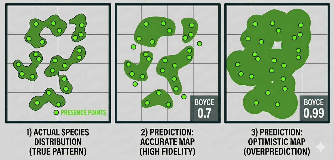
Figure: Boyce index and overprediction. Generated with Google Gemini.

An alternative approach frequently used is to calculate standard binary metrics by using presence points alongside background data (points randomly sampled from the study area) as a proxy for absences. However, this method introduces significant uncertainty (Soley-Guardia et al. 2024), as the statistical bias resulting from the lack of true absences makes it difficult to distinguish whether a high score reflects actual model accuracy.