
| LM | Sample Presence-Absence Points |
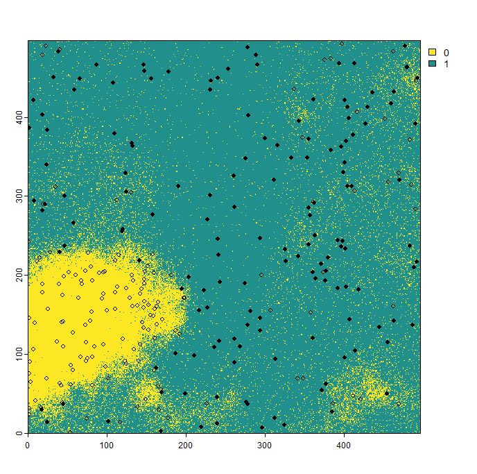
For this course, we want to sample presence-absence points instead of presence-only points for all virtual species. We will again use the virtualspecies R package for this. The function sampleOccurrences can be used to do this task. It allows you to define how many points (n) you want to sample, and whether you want to sample the same number of presence and absence data points, which is referred to as sample prevalence.
The sample prevalence is a number between 0 and 1. Higher values indicate a larger proportion of presence data in the presence-absence dataset. You can see the results in the image below.
Restricting sampling areas
Apart from adjusting sample prevalence and the number of points to be sampled, many more options are available to customize the sampling of presence-absence data. In real-world scenarios, it is highly unlikely that the entire study area will be sampled. Most of the time, sampling is limited to specific regions. To demonstrate this, we will restrict our sampling area using the blockCV R package (Valavi et al. 2019).
The blockCV package is primarily designed for spatial cross-validation which means it can be used for creating spatial blocks around presence-only or presence-absence data. This makes it also a good tool for defining polygons for biased sampling of presence-absence data. To achieve this, we will first sample random background points across the study area and then create spatial blocks. Several options for block shapes are available, as shown in the image below. We will create polygons using squares, hexagons, and bars across the study area. The size argument allows you to specify the size of each individual block.
In the following figure, you can see the results of using different polygon shapes to create spatial blocks across the study area.
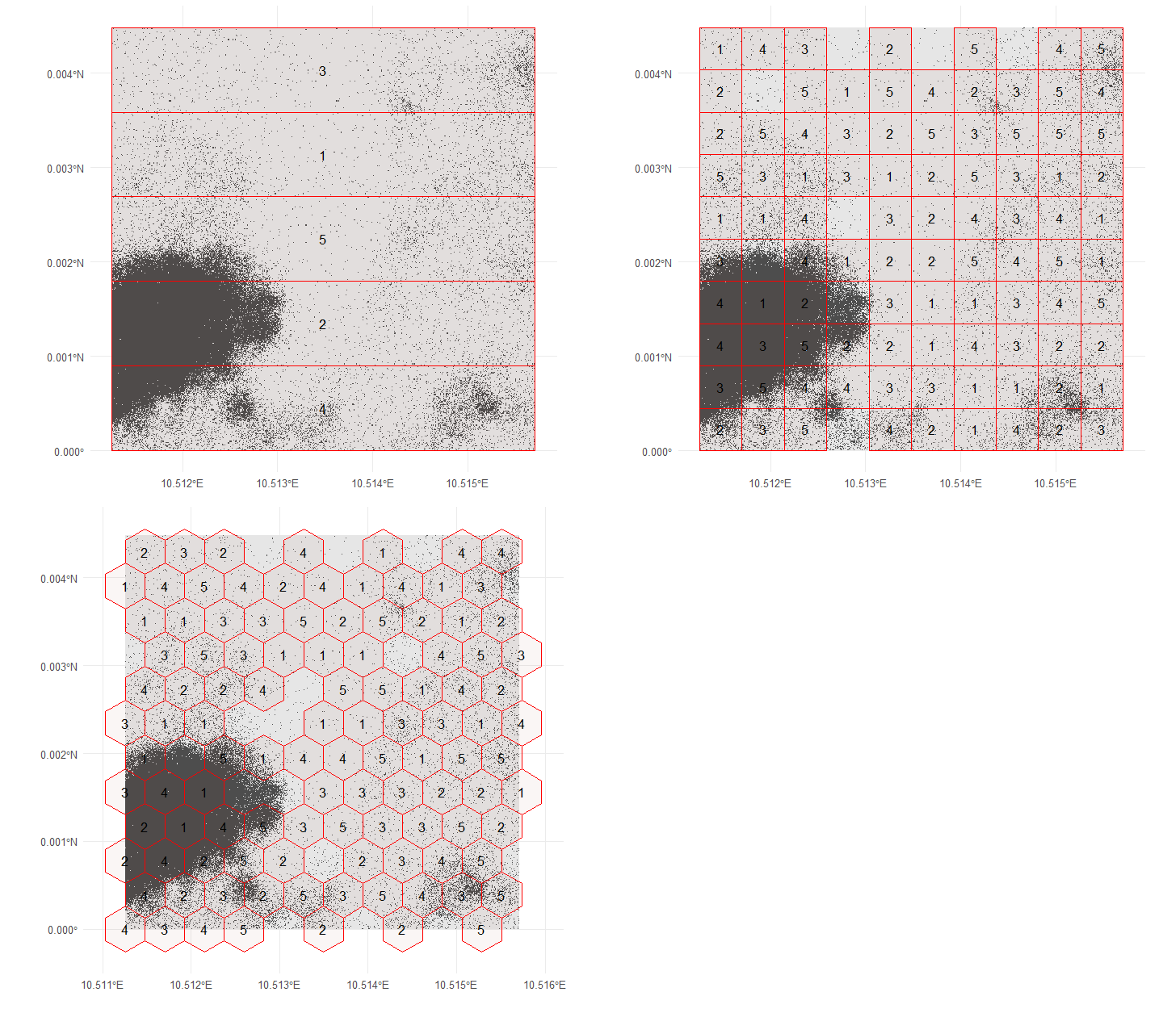
Most of the time, real-world sampling areas are not perfectly symmetrical. You could use tools like QGIS to draw custom polygons that result in less symmetrical shapes. In this session however, we will use the last block type, hexagons, to sample our presence-absence points in just a few regions. For this, we use the polygons created with the blockCV package and sample occurrences only within a subset of these polygons.

Introducing further sampling bias
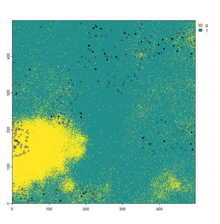
We will introduce two additional sampling biases into our presence-absence sampling strategy for the virtual species. First, we will incorporate the probability of detecting a species. This means that for species that are difficult to survey, absence points may still be recorded even if the species is actually present in the area. This reflects real-world conditions, particularly for mobile species such as birds or bats. In such cases, the statement “absence of evidence is not evidence of absence” applies.
If the detection probability is set to zero, the species cannot be detected at all. Conversely, if it is set to one, the species is always detected. In the example below, we demonstrate the results for a relatively low detection probability of 0.3. As shown, the species is often recorded as absent in areas where it is actually present.
The second sampling, as seen in the code above, represents the error probability. This reflects potential errors that can occur during field sampling, where a species is not actually present but is incorrectly recorded as present in the dataset. Including this error probability in your dataset may result in output like the following (red rows in the table):
| x | y | Real | Observed |
|---|---|---|---|
| 239.5 | 400.5 | 1 | 1 |
| 460.5 | 446.5 | 0 | 0 |
| 427.5 | 156.5 | 1 | 0 |
| 153.5 | 313.5 | 0 | 0 |
| 387.5 | 134.5 | 0 | 0 |
| 259.5 | 475.5 | 1 | 1 |
| 241.5 | 33.5 | 0 | 1 |
| 175.5 | 331.5 | 0 | 1 |
| 153.5 | 313.5 | 0 | 0 |
Table: The row highlighted in blue indicates a low detection probability, resulting in the species being present but undetected. Rows highlighted in red indicate detection errors where the species is absent but incorrectly recorded as present.