LM Virtual species

Here, you’ll learn how to generate virtual species for modeling purposes, which will later allow us to conduct a comprehensive comparison of species distribution models.

„Species distribution models (SDMs) have become one of the major predictive tools in ecology. However, multiple methodological choices are required during the modelling process, some of which may have a large impact on forecasting results. In this context, virtual species, i.e. the use of simulations involving a fictitious species for which we have perfect knowledge of its occurrence–environment relationships and other relevant characteristics, have become increasingly popular to test SDMs. This approach provides for a simple virtual ecologist framework under which to test model properties, as well as the effects of the different methodological choices, and allows teasing out the effects of targeted factors with great certainty. This simplification is therefore very useful in setting up modelling standards and best practice principles.” (Meynard et al. 2019)

As described in the excerpt above from the 2019 study by Meynard et al. virtual species have become an important tool today to evaluate and test species distribution models. To date, there are several frameworks that can be used to create virtual species. For example:

virtualspecies (Leroy et al. 2016)
sdmvspecies (Duan et al. 2014)
nicheA (Qiao et al. 2015)

The first two are R packages, while NicheA is a standalone Java platform. In this session, we will use the R package virtualspecies (Leroy et al. 2016) along with previously designed neutral landscape models (NLMs) to generate virtual species distributions. The virtualspecies R package provides several methods for creating virtual species distributions, including approaches where species distributions are generated either completely at random or by defining the relationship between environmental variables through specific functions. The latter approach is more customizable but also more time consuming as the relationship of the species to each variable needs to be defined first. For those interested in a comprehensive guide, the online tutorial for the package provides more detailed instructions, as only a small portion of its functionality will be covered in this course.

The general workflow that involves creating virtual species can be found in the figure below. It provides the comprehensive workflow of creating virtual species from scratch. As we only have limited time in this course, we will not be able to deal with all parts of it.

Image: Stages involved in the simulation of a virtual species. Image from Meynard et al. 2019.

Creating random virtual species

When creating virtual species, several factors can significantly impact the results and subsequent testing of SDMs. Considerations include:

Niche Breadth: Does the virtual species occupy a broad or narrow ecological niche? It is a good idea to have several species with different niche breadth.
Sampling Strategy: How were presence-absence points sampled? Was a sampling bias introduced, or were points sampled evenly across the landscape?
Presence-Absence Conversion: How is the probability of occurrence converted to presence-absence maps? This is particularly crucial because methods used to set thresholds for presence-absence can influence model outcomes greatly.

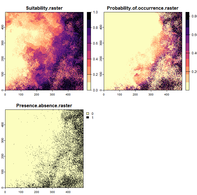
We will begin by creating a simple, randomly generated virtual species. This function employs standard settings to generate a species using a principal component analysis (PCA) from the environmental variables. By default, it also produces a presence-absence map for the species, utilizing the “probability” functionality where probabilities of occurrence are transformed with a logistic function. Alternatively, you can set a simple threshold to transform the probability, where values below the threshold indicate absence and values above it indicate presence. However, it has been shown that this threshold-based approach can produce unrealistic species distributions, as real species may be absent from highly suitable areas or present in less suitable areas due to factors like biotic pressures or microclimatic conditions. For further information, refer to the dedicated tutorial chapter by Boris Leroy or the paper by Meynard et al. (2019).

As a result, three rasters are generated: suitability, probability of occurrence, and presence-absence rasters, as shown in the figure below. You can adjust the niche breadth to narrow to observe how this affects the results. It is also possible to select specific raster layers to create a random species based solely on these selected layers.

Create virtual species by defining response functions

The second, more complex way to define virtual species is by specifying the response of the species to each variable individually. The simplest way to illustrate this concept is with an example involving temperature. For instance, we could assume a linear relationship between the habitat suitability of the species and temperature, such that as the temperature increases, the habitat becomes less suitable for the species. However, other types of relationships are also conceivable. For example, there might be an optimal temperature range for the species, where temperatures that are too high or too low make the habitat unsuitable.

By defining these relationships, we can model different ways species respond to environmental variables. The virtualspecies package provides several built-in functions to simulate these species’ responses to different variables. To achieve this, the variables are transformed using a function.

Available transformations of environmental variables:

Linear function: Assumes a direct relationship between the variable and suitability.
Quadratic function: Models a peak or trough in the response.
Logistic function: Creates an S-shaped curve, often used for threshold responses.
Beta response functions: Allows for a more flexible bell-shaped curve.
Normal distribution: Models a symmetrical response around an optimal value.
Custom function: You can define your own mathematical function for transformations.

The figure below demonstrates how these functions can transform the environmental variable NLM1 created in the previous session.

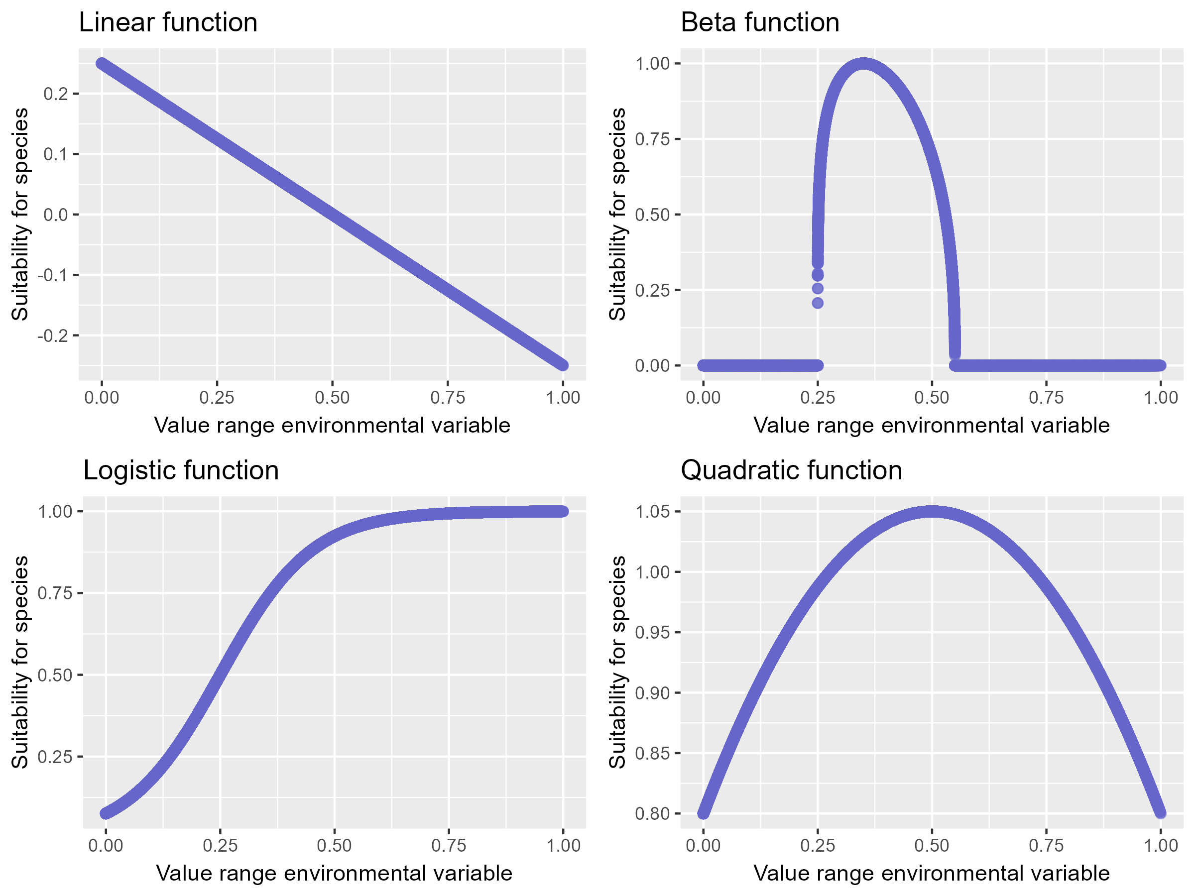Image: : The values of the variable NLM1 transformed with a linear, beta, logistic and quadratic function.

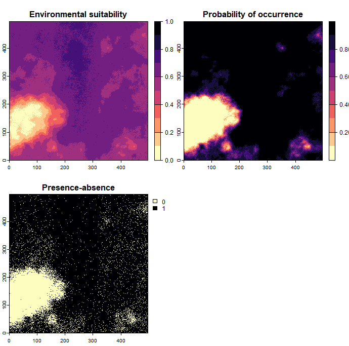
In this section, we will create a virtual species by defining its response to environmental variables using a custom function. To do this, we first use the function formatFunction to define how each environmental variable influences the species. You can work with one variable or multiple variables, but keep in mind that the more variables you include, the more complex it becomes to ensure that their suitability values do not contradict each other. Once the response functions are defined, we then specify a formula that determines how strongly each variable influences the habitat suitability of the species. This part is highly flexible, allowing you to be creative with how you combine the environmental variables. However, be sure that the variables you use in the formula correspond to the variables defined in the raster stack provided to the function and are consistent with the parameters you set.

The generateSpFromFun function does not automatically convert suitability values into presence-absence maps. To obtain the same output as with the generateRandomSp function, we use the convertToPA function for this conversion:

Creating random virtual species

Create virtual species by defining response functions

Available transformations of environmental variables:

Further reading