Ex Artificial landscapes

Exercise: Create Environmental Variables

Now it’s your turn! Use the code in the gist below to generate six different environmental variables. Ensure each variable has the same spatial extent so they can be combined into a single raster stack.

If any layers have a larger extent, use the function terra::crop to adjust them to the target area. Once all layers are aligned, save them as a single .tif file for easier access and sharing.

Note: NLMR has no support for the terra package yet, therefore we will transform each of the NLMs to a spatRaster after creating it.

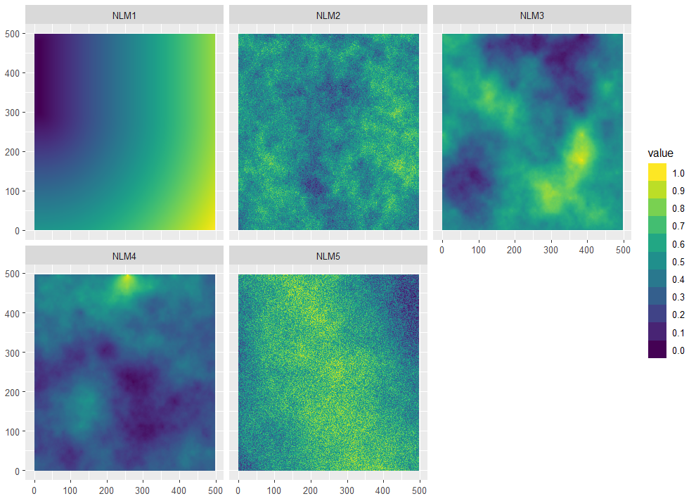
Once completed, you’ll have a comprehensive environmental dataset ready for analysis or modeling. Your dataset look somewhat like the one in the following figure (continuous variables plotted with tidyterra as explained in Unit 01 ):

Additional learning material: Multicorrelinarity between environmental variables

In ecological modeling, researchers frequently incorporate a substantial number of environmental variables. In Species Distribution Modeling the number of variables can easily exceed 100 variables (e.g., Bald et al. 2024). This can quickly lead to a situation in which two or more predictor variables in a model are highly correlated, meaning that they provide redundant information about the variance in the outcome. This phenomenon, known as collinearity, is prevalent in ecological and environmental studies, particularly among interrelated variables such as temperature, precipitation, and humidity.

Collinearity can affect model performance by inflating metrics, which may result in the incorrect identification of important environmental predictors (Dormann et al. 2012). Consequently, it is advisable to evaluate the correlation among variables prior to model development. This can be done with a simple function in R. As a result, you will get a correlation matrix which shows you the positive and negative correlations between variables, along with their respective strengths. To mitigate the impact of collinearity, it is advisable to establish a threshold, (e.g., 0.8), and to exclude variables that exceed this threshold.

For further insights into the implications of collinearity in ecological modeling, refer to the study by Dormann et al. (2012).

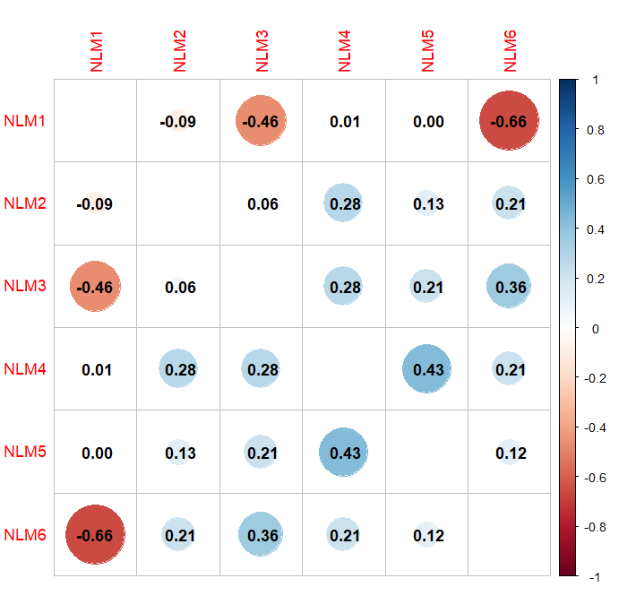
You can use the script below to create a correlation matrix for the six NLMs we created in the esxercise above.

In the end your confusion matrix should look like this:

Exercise: Create Environmental Variables

Additional learning material: Multicorrelinarity between environmental variables

Further reading: