Predicting time series
Time-series analyses can generally be divided into forecasting future dynamics and describing and potentially explaining past patterns. Since the latter often requires continuous i.e. gap-free observations, we start with a simple forecasting procedure, which can also be used for gap-filling in some cases.
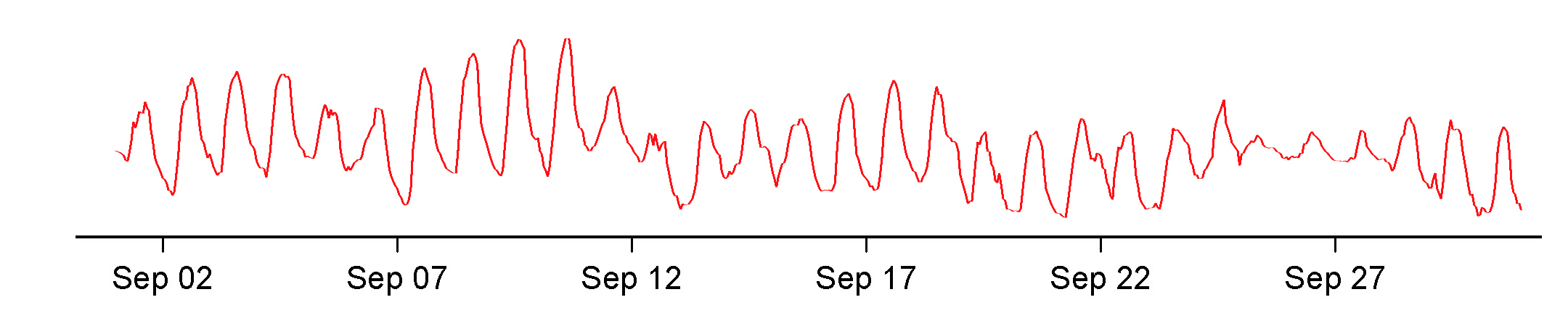
To illustrate forecasting, we will again use the (mean monthly) air temperature records of the weather station in Cölbe (which is closest to Marburg). The data has been supplied by the German Weather Service.
# read data we saved in the last session
tam <- read.table("tam.txt", header = TRUE, sep = ";")
head(tam)
##     Date        Ta
## 1 200607 21.753970
## 2 200608 15.567473
## 3 200609 16.683194
## 4 200610 12.118817
## 5 200611  7.325556
## 6 200612  4.468011
Auto-regressive and moving average models for predicting time series
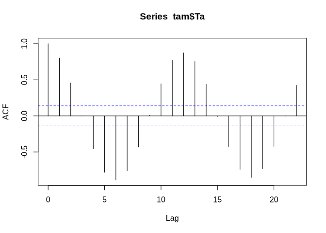
In order to predict the time series just based on its observed dynamics, an auto-regressive integrated moving average model (ARIMA) can be used. ARIMA is not a diagnostic model for the identification of seasonal or other periodic components. On the contrary, it requires a stationary time series, which is a prerequisite we already know is not true for the monthly mean air temperature values between July 1st 2006 and December 31st 2022.
acf(tam$Ta)
Auto-regressive models (AR)
While we could start with de-trending and de-seasoning now, let us try a quick-and-dirty approach first and postpone the time series decomposition to the next session. One thing one could try is to not use the original values but the difference between the consecutive value pairs (i.e. the difference between time t and t+1 etc.). And if one difference is not enough, we can compute the differences of the differences and the auto-correlation behaviour would look like this:
dTa <- diff(diff(tam$Ta))
acf(dTa)
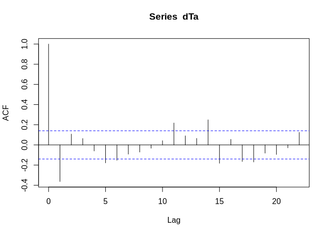
Not perfect but good enough to be used in this example. Before we run the ARIMA model, we run a simple AR model first:
armod <- ar(dTa, aic = TRUE, order.max = 20, method = "yule-walker")
armod
##
## Call:
## ar(x = dTa, aic = TRUE, order.max = 20, method = "yule-walker")
##
## Coefficients:
##       1        2        3        4        5        6        7        8
## -0.8578  -0.5895  -0.3433  -0.2797  -0.4231  -0.5408  -0.5385  -0.4862
##       9       10       11       12       13       14
## -0.4245  -0.2970  -0.0344   0.0963   0.1368   0.2154
##
## Order selected 14  sigma^2 estimated as  8.14
The ar function computes an AR model and iterates over the lags to be included in the linear equation,
which predicts the monthly air temperature values for time t based on its value at time t-1, t-2, and so on.
The maximum number of lags (within a maximum of 20 as provided to the function) is determined based on an internal estimate of the AIC parameter. The number of lags with the minimum AIC are used:
plot(0:20, armod$aic, type = "o")
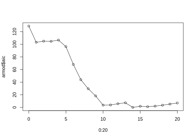
Using the Yule-Walker method for estimating the AR parameters, a maximum lag of 14 is considered. Although the results will be quite different if another method is used and although the following is of no use if one actually wants to use not just an AR or a MA but an ARIMA model, a rule of thumb states that if
- the auto-correlation function declines exponentially or shows a sinus pattern and
- the partial auto-correlation function shows only p significant lags in the beginning,
an AR(p) model (i.e. an AR model with p considered lags) is a good starting point. In the auto- and partial auto-correlation function of the two-times differentiated dataset, we might see exactly this:
par_org <- par()
par(mfrow = c(1,2))
acf(dTa)
pacf(dTa)
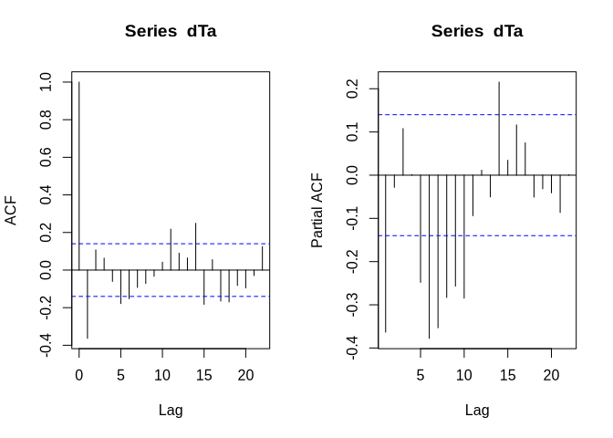
par(par_org)
If we change the parameter estimation method, the results look like this (16 instead of 14 is the optimum now):
armod <- ar(dTa, aic = TRUE, order.max = 20, method = "mle")
armod
##
## Call:
## ar(x = dTa, aic = TRUE, order.max = 20, method = "mle")
##
## Coefficients:
##       1        2        3        4        5        6        7        8
## -1.5912  -2.0621  -2.3764  -2.6146  -2.8816  -3.0777  -3.1469  -3.1423
##       9       10       11       12       13       14       15       16
## -3.0874  -2.9369  -2.5753  -2.1653  -1.6939  -1.0681  -0.6365  -0.2034
##
## Order selected 16  sigma^2 estimated as  3.39
So the optimal value for the lag parameter depends on the chosen method.
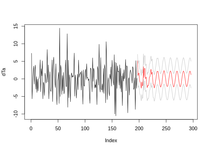
Let us now use th AR model for predicting the time series into the future (although 100 months in the future is way to much; grey lines indicate the standard error):
arpred <- predict(armod, n.ahead = 100)

plot(dTa, type = "l", xlim = c(0, length(dTa)+100))
lines(arpred$pred, col = "red")
lines(arpred$pred + arpred$se, col = "grey")
lines(arpred$pred - arpred$se, col = "grey")
Auto-regressive integrated moving average models (ARIMA)
The above AR model examples are mainly for illustration purposes and have low predictive power. The predictive power increases with combining the AR model part with a moving average model (MA) - ARIMA.
In the ARIMA world, three parameters are generally required:
- p which is the number of time lags considered in the AR model,
- d which is the number of differences taken from the dataset (to reach stationarity), and
- q which is the number of time lags considered in the MA model.
Hence, if we want to compute an ARIMA comparable to the AR above (the second one), we call it with:
armod <- arima(tam$Ta, order = c(16,2,0), method = "ML")  # the order is p, d, q
armod
##
## Call:
## arima(x = tam$Ta, order = c(16, 2, 0), method = "ML")
##
## Coefficients:
##           ar1      ar2      ar3      ar4      ar5      ar6      ar7      ar8
##       -1.5905  -2.0603  -2.3734  -2.6106  -2.8770  -3.0727  -3.1417  -3.1373
## s.e.   0.0708   0.1274   0.1809   0.2178   0.2424   0.2597   0.2684   0.2715
##           ar9     ar10     ar11     ar12     ar13     ar14     ar15     ar16
##       -3.0825  -2.9320  -2.5703  -2.1606  -1.6898  -1.0649  -0.6344  -0.2024
## s.e.   0.2712   0.2677   0.2595   0.2416   0.2165   0.1797   0.1265   0.0707
##
## sigma^2 estimated as 3.394:  log likelihood = -405.08,  aic = 844.15
Finding the right values for an ARIMA model is not trivial. Basically, one has to iterate over a variety of options. Let us try just one for illustration purposes.
arimamod <- arima(tam$Ta, c(6,2,2))
summary(arimamod)
##
## Call:
## arima(x = tam$Ta, order = c(6, 2, 2))
##
## Coefficients:
##          ar1     ar2     ar3      ar4      ar5      ar6      ma1     ma2
##       0.3725  0.0823  0.0408  -0.1707  -0.3006  -0.2665  -1.9114  0.9152
## s.e.  0.0739  0.0717  0.0715   0.0716   0.0726   0.0741   0.0376  0.0374
##
## sigma^2 estimated as 3.976:  log likelihood = -421.01,  aic = 860.01
##
## Training set error measures:
##                     ME     RMSE      MAE      MPE     MAPE      MASE
## Training set 0.2484168 1.983889 1.596457 33.56211 59.27694 0.4886506
##                     ACF1
## Training set -0.03297744
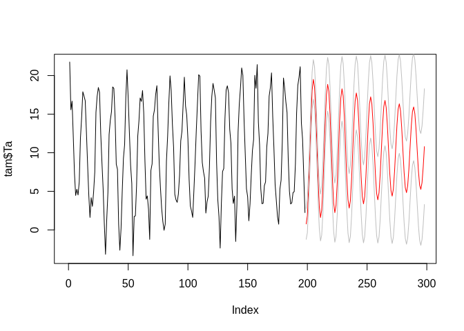
We will not focus on optimal prediction in this example, so these results are just fine for the purpose of illustration. The ARIMA model can be used to predict the time series in the future analogously to the AR model:
arima_predict <- predict(arimamod, n.ahead = 100)

plot(tam$Ta, type = "l", xlim = c(0, length(dTa)+100))
lines(arima_predict$pred, col = "red")
lines(arima_predict$pred + arima_predict$se, col = "grey")
lines(arima_predict$pred - arima_predict$se, col = "grey")
Finding the right parameters for ARIMA
Finding the right number of lags p for the AR model, number of differentiations d, and number of lags q for the MA model requires several iterations.
You now already know everything you need to e.g. iterate over a bunch of values for each parameter and select the appropriate combination by minimizing e.g. cross-validation errors.
An alternative approach could be the forecast::auto.arima function.
It iterates over the parameters (see defaults of the function) and applies some statistical tests for e.g. stationarity.
It will also include seasonal components in the ARIMA model
(which is basically the same as a time lag but with respect to the seasonal difference, e.g. a seasonal component [12] with a lag of 1 skips 12 months, one for [4] would skip a quarter of a year).
Finding the right parameters for ARIMA with the auto.arima function
The forecast package generally works on time series data of class ts, which is easy to generate if you actually have a complete (i.e. gap-free) time series. The time series is defined by the values, the starting point in time (e.g. year and month), the end point in time, the frequency of observations per main time unit and the time step delta t.
For monthly data starting in July 2006 and ending in December 2022, the creation of a time series looks like this:
tam_ts <- ts(tam$Ta, start = c(2006, 7), end = c(2022, 12),
             frequency = 12)
str(tam_ts)
## Time-Series [1:198] from 2006 to 2023: 21.75 15.57 16.68 12.12 7.33 ...
Now we can use the forecast::auto.arima function. We will extend the iteration over p and q to 20 to be compatible with the above example but we will not include a seasonal component for the moment:
arima_ns <- forecast::auto.arima(tam_ts, max.p = 20, max.q = 20, stationary = TRUE, seasonal=FALSE)
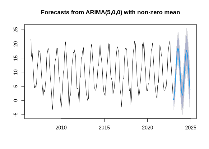
summary(arima_ns)
## Series: tam_ts
## ARIMA(5,0,0) with non-zero mean
##
## Coefficients:
##          ar1     ar2     ar3      ar4      ar5    mean
##       0.5127  0.1307  0.0213  -0.2077  -0.4097  9.9924
## s.e.  0.0658  0.0748  0.0751   0.0753   0.0665  0.1528
##
## sigma^2 = 4.235:  log likelihood = -423.34
## AIC=860.68   AICc=861.27   BIC=883.7
##
## Training set error measures:
##                     ME     RMSE      MAE     MPE    MAPE      MASE       ACF1
## Training set 0.0246255 2.026541 1.597263 38.3537 71.5643 0.8362305 -0.0825803
Actually, the ARIMA model comes with d = 0, which means that the data values are not differentiated (which is a tough choice).
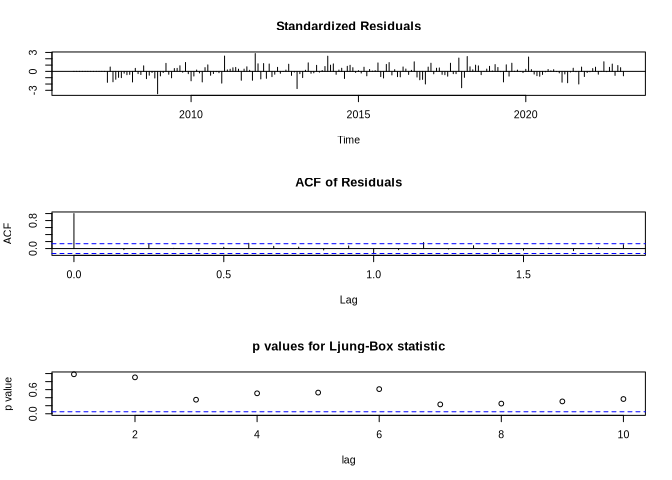
To better estimate the quality of the ARIMA model, we can use some diagnostic plots:
tsdiag(arima_ns)
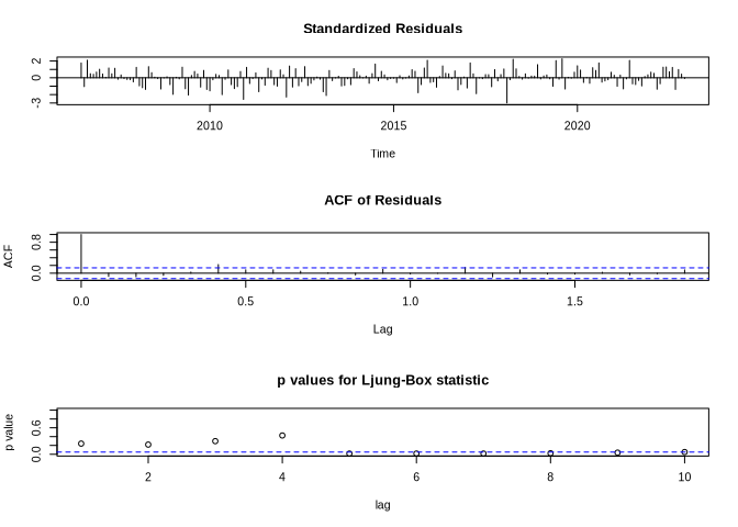
The last plot shows test results if the residuals were independently distributed. For time lags larger than 4, this may not be the case, which indicates that the ARIMA model is not really well specified.
The forecast looks like this:
plot(forecast::forecast(arima_ns))
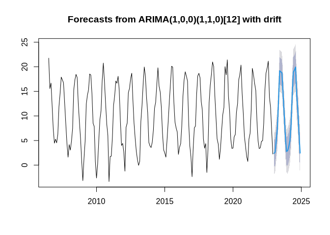
If we include a seasonal component, the results look like this:
arima_s <- forecast::auto.arima(tam_ts, max.p = 20, max.q = 20, seasonal=TRUE)
summary(arima_s)
## Series: tam_ts
## ARIMA(1,0,0)(1,1,0)[12] with drift
##
## Coefficients:
##          ar1     sar1    drift
##       0.1211  -0.5211  -0.0025
## s.e.  0.0733   0.0637   0.0099
##
## sigma^2 = 4.568:  log likelihood = -405.6
## AIC=819.2   AICc=819.42   BIC=832.11
##
## Training set error measures:
##                       ME    RMSE      MAE       MPE     MAPE      MASE
## Training set -0.03883731 2.05483 1.544685 -2.425242 41.78898 0.8087037
##                    ACF1
## Training set 0.00160073
tsdiag(arima_s)
plot(forecast::forecast(arima_s))
So which parameter combination is the best? You will tackle this question with the assignment of this unit.