
Maps
Introduction
Here, we will process, visualize, and transform spatial data.
Raster Data and Common Formats
Raster data represents spatial data as a grid of cells or pixels, where each cell has a specific value. This type of data is typically used for continuous variables such as elevation, temperature, or satellite imagery. Raster data is particularly useful for analyzing large-scale spatial patterns and performing environmental modeling.
Common Raster Formats:
- GeoTIFF (.tif, .tiff) – A widely used format that supports metadata and multiple bands.
- ASCII Grid (.asc) – A text-based raster format, often used in GIS applications.
Packages to handle tiff data are for example terra and raster.
The geodata-package provides access to different spatial data
library(terra)
library(geodata)

# Download population data
population <- population(2020, 5, path = "Data")
plot(population)
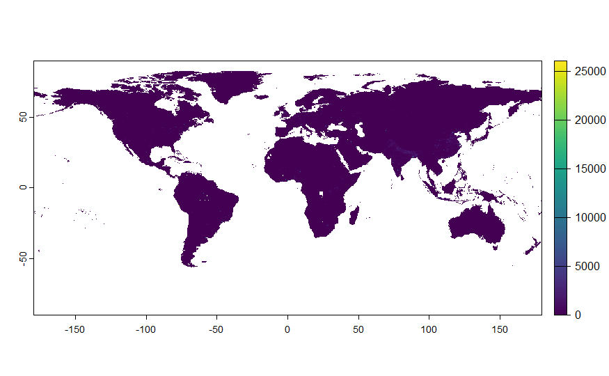
We see that this function saves data in .tif format.
Vector Data and Common Formats
Vector data represents geographic features using points, lines, or polygons. This type of data is suited for discrete features such as roads, administrative boundaries, or specific locations.
Types of Vector Data:
- Point Data – Represents specific locations (e.g., weather stations, city centers).
- Line Data – Represents linear features (e.g., roads, rivers, power lines).
- Polygon Data – Represents areas (e.g., country borders, lakes, land use zones).
Common Vector Formats:
- Shapefile (.shp, .dbf, .shx, .prj) – A widely used format consisting of multiple files:
.shp(geometry),.dbf(attributes),.shx(spatial index), and.prj(projection metadata). The absence of a.prjfile can result in CRS ambiguity. - GeoJSON (.geojson) – A JSON-based format designed for web applications, supporting multiple geometry types and embedded CRS.
- KML (.kml) – Often used in Google Earth, this format supports both spatial features and visualization attributes.
- CSV with Coordinates – A tabular format where latitude and longitude values represent spatial locations; it typically lacks explicit CRS metadata.
R provides several packages for handling vector data, such as sf and sp.
Again, we’ll use geodata to get some spatial data, in this case vector data. However, when we have a look at the location where the data was downloaded we see that it’s not saved in one of the mentioned data formats. We’ll thus export it to make it easier to share:
library(sf)

# Load administrative boundaries of Germany
germany <- geodata::gadm(country="Germany", path="Data", level=2)
plot(germany)

# Save as Shapefile
writeVector(germany, "germany_boundaries.shp", overwrite=TRUE)
Projection Systems and Coordinate Reference Systems (CRS)
Raster and vector datasets do not inherently have a spatial reference system unless it is explicitly defined. Formats such as GeoTIFF and Shapefile support CRS metadata, which is crucial for aligning spatial data from different sources. Without proper CRS definitions, datasets may not overlay correctly in a GIS environment.
A Coordinate Reference System (CRS) defines how spatial data is projected onto a two-dimensional surface.
Types of Projection Systems:
- Geographic Coordinate Systems (GCS) – Uses latitude and longitude (e.g., WGS84, EPSG:4326).
- Projected Coordinate Systems (PCS) – Projects the Earth’s surface onto a flat plane (e.g., UTM, EPSG:32633 for UTM Zone 33N).
here’s how you can assess which projection a map has:
st_crs(germany) # Prints the CRS of the Germany shapefile
Example of applying projections in R:
# Convert to sf
germany_sf <- st_as_sf(germany)

# Transform from WGS84 to UTM Zone 33N
germany_utm <- st_transform(germany_sf, crs = 32633)
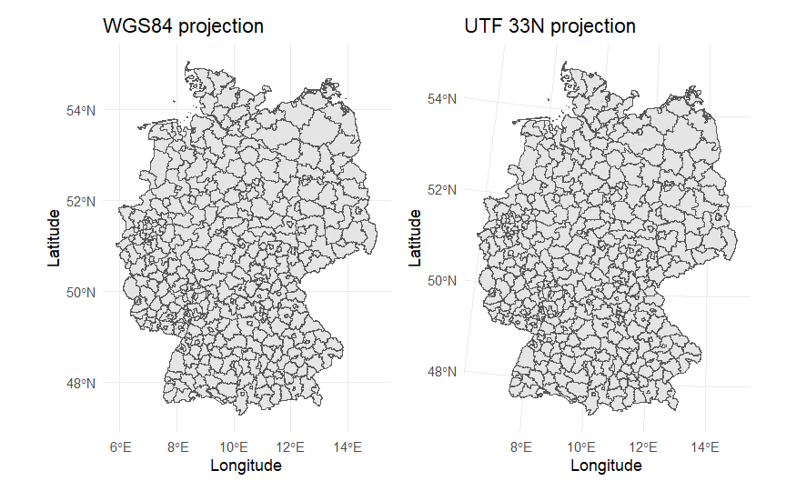
Let’s see how it looks like in both projections projection
library(ggplot2)
library(patchwork)

wgs <- ggplot() +
  geom_sf(data = germany_sf) +
    labs(title = "WGS84 projection",
       x = "Longitude", y = "Latitude") +
  theme_minimal()
utf <- ggplot() +
  geom_sf(data = germany_utm) +
    labs(title = "UTF 33N projection",
       x = "Longitude", y = "Latitude") +
  theme_minimal()

wgs+utf
Mapping Hessen and Universities
Here, we’ll walk through how we’re mapping the Universities of hessia:
First, we extract Hessia as region from the overall data set and create a data set of the location and number of students of universites:
# Extract only Hessen
hessen <- germany[germany$NAME_1 == "Hessen", ]

# Create a dataset of universities
hessian_universities_state <- data.frame(
  University = c(
    "Johann Wolfgang Goethe-Universität Frankfurt am Main",
    "Justus-Liebig-Universität Gießen",
    "Technische Universität Darmstadt",
    "Philipps-Universität Marburg",
    "Universität Kassel",
    "Technische Hochschule Mittelhessen (THM)",
    "Frankfurt University of Applied Sciences",
    "Hochschule Darmstadt",
    "Hochschule RheinMain",
    "Hochschule Fulda",
    "Hessische Hochschule für Polizei und Verwaltung Wiesbaden",
    "Hochschule Geisenheim University",
    "Hessische Hochschule für Finanzen und Rechtspflege Rotenburg",
    "Hochschule des Bundes für öffentliche Verwaltung"
  ),
  Students = c(
    41107, 25461, 24008, 21237, 20898, 15792, 15038, 14377, 12271, 8682,
    4299, 1595, 1498, 1357
  ),
  Latitude = c(
    50.1272, 50.5831, 49.8728, 50.8019, 51.3127,
    50.5722, 50.1205, 49.8682, 50.0827, 50.5529,
    50.0782, 49.9869, 50.9975, 50.7381
  ),
  Longitude = c(
    8.6696, 8.6784, 8.6512, 8.7744, 9.4797,
    8.6671, 8.6596, 8.6431, 8.2322, 9.6823,
    8.2398, 7.9736, 9.7331, 7.8982
  )
)
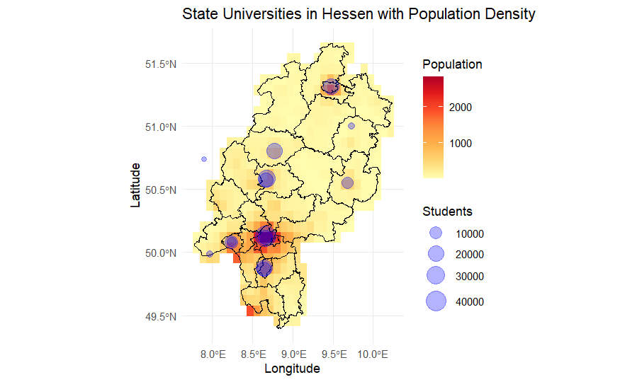
Creating the Map
Now, we use ggplot2 to visualize the data. The base map will show the population as a raster layer, with universities added as points.
First, we need to reduce the population raster to Hessia
# Clip raster precisely to Hessen boundaries
population_hessen <- terra::crop(population, terra::ext(hessen))
population_hessen <- terra::mask(population_hessen, hessen)
crop(population, ext(hessen)) crops the raster to the bounding box of Hessen, but does not precisely cut along the polygon edges. mask(population_hessen, hessen, exact=TRUE): Ensures raster cells are trimmed exactly along Hessen’s boundary, rather than keeping entire intersecting cell
It does not however, lead to smooth edges.
buidling the map using ggplot2:
# Convert population raster to a data frame for ggplot
pop_df <- as.data.frame(population_hessen, xy = TRUE)
colnames(pop_df) <- c("Longitude", "Latitude", "Population")

# Remove NA values
pop_df <- na.omit(pop_df)


# Plot the map
ggplot() +
  # Add population raster
  geom_raster(data = pop_df, aes(x = Longitude, y = Latitude, fill = Population)) +
  scale_fill_distiller(palette = "YlOrRd", direction = 1) +

  # Add Hessen boundaries
  geom_sf(data = st_as_sf(hessen), fill = NA, color = "black", size = 0.5) +

  # Add universities as points
  geom_point(data = hessian_universities_state,
             aes(x = Longitude, y = Latitude, size = Students),
             color = "blue", alpha = 0.3) +

  # Adjust size scale
  scale_size(range = c(2, 8), name = "Students") +

  # Labels
  labs(title = "State Universities in Hessen with Population Density",
       x = "Longitude", y = "Latitude") +

  # Add theme
  theme_minimal() +
  theme(legend.position = "right")
Here’s a way to actually get smooth eges, but it takes some time: ```{r eval=FALSE, include=TRUE}
Clip raster to Hessen# Convert raster to polygons
population_hessen_poly <- as.polygons(population, trunc=FALSE, dissolve=TRUE)
Clip it precisely using Hessen’s boundary
population_hessen_clipped <- st_intersection(st_as_sf(population_hessen_poly), st_as_sf(hessen))
plot(population_hessen_clipped)
---

### **Linking Population Data to Municipalities**
In this example we'll have a look on how to add data to an existing vector layer. First, we'll create a dataset. Data was taken from Daten https://statistik.hessen.de/unsere-zahlen/bevoelkerung, © Hessisches Statistisches Landesamt, Wiesbaden, 2024
```{r}
age <- data.frame(NAME_2 = hessen$NAME_2,
                  population = c(274484,164832,302263,749596,222688,268141,267920,118010,240622, 230742,197065, 254444,174281,419055,238593,243093,94246,356578,131845,186050,180368,101494,155135,98055,310705,287241),
                  under3=c(7333,4389, 7986, 22223, 6145,7232,8146,3030, 5739,5826,5456,6843,4665,11983,6511,6091, 2373,10137,4307,4519,4502,2550,3886, 2359,8376,8198))

age$proportion <- age$under3/age$population

hessia <- st_read("germany_boundaries.shp")
When a Shapefile is read using the sf package in R, it is stored as an sf (Simple Features) object. This object contains:
Geometry (sfc column): Stores the spatial features (points, lines, or polygons). Attributes (data frame columns): Stores non-spatial data, such as names, population, or any other metadata. Coordinate Reference System (CRS): Specifies the spatial reference system used for georeferencing. Bounding Box (bbox): Defines the extent of the dataset. Feature Type: Describes whether the geometry consists of points, lines, or polygons.
We can merge external data if theres a matching attribute, just as we would do with normal data frames.
hessia_age <- merge(hessia, age, by = "NAME_2")
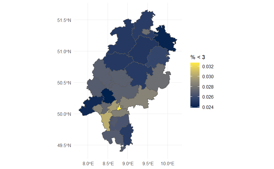
# Plot the percentage of children under 3 years
library(ggplot2)
ggplot() +
geom_sf(data = hessia_age, aes(fill = proportion)) +
scale_fill_viridis_c(option = "cividis", name = "% < 3") +
theme_minimal()
This project demonstrates geospatial data processing in R, including projections, spatial data manipulation, and visualization using real-world data from Hessen, Germany.