| LM | Deeply good |
This learning module focuses (once again) on predicting spatial structures. In the previous unit, we saw that random forest models are capable of making good predictions at the pixel level. Yet we are interested in identifying spatial structures in their entirety. In this case, the value of a single pixel is interesting, but the values of a neighborhood of pixels is much more interesting. Deep learning neural networks are appropriate for recognizing structures in this way.
Deep learning in a nutshell
If this is your first exposure to deep learning, this section serves as an incredibly brief introduction to the world of neurons. If you are already familiar with the concept of deep learning neural networks, you can skip ahead directly to the U-Net section.

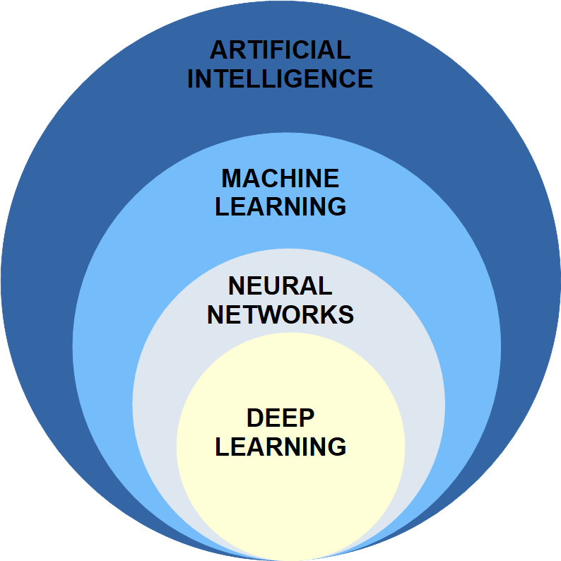
Deep learning algorithms are a machine learning tool, just like random forest models. Deep learning is a special form of neural networks, as we can see in the image above, that are used frequently e.g. in computer vision. In the video below some operations were mentioned, that are used in the calculation of CNNs to transform the data, which are not explained in depth in this module. These also partially represent hyperparameters that are in the code of the exercises that occur in this unit. For a deeper understanding and the mathematical basics see: Dumoulin and Visin (2018) , Nielsen (2015) and StatQuest.
U-Net
The following exercises will use a U-Net convolutional neural network to recognize spatial structures. Originally, the technique was developed to segment biomedical images. U-Net performs a semantic segmentation, in which each pixel is assigned to a class. For a short introduction, have a look at the U-Net teaser: 5 Minute Teaser Presentation of the U-net: Convolutional Networks for Biomedical Image Segmentation (5:03)
The network structure
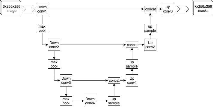
The image below is an example of a U-Net. We can see that the input into the U-Net is an image (256 x 256) with three layers. A convolution (e.g., 3x3) is applied to this input image, sometimes even several times in succession. From that point, a step called downsampling starts, which is performed by a max pooling operation. In this process, the spatial information becomes weaker, but the information content about what is being depicted in the image becomes increasingly larger. Subsequently, to generate information about the space, a transposed convolution applies an upsampling. This step uses half of the neurons from the left side and takes the other half from the upsampling. The final step is a 1x1 convolution, which gives the segmented output.
This and further information can be found in the paper on the U-Net algorithm: Ronneberger et al. (2015) U-Net: Convolutional Networks for Biomedical Image Segmentation.
 Image: Example architecture of U-Net for producing k 256-by-256 image masks for a 256-by-256 RGB image. Mehrdad Yazdani [CC BY-SA 4.0] via wikipedia.org
Unit 4 slides
Further reading
Goodfellow, I., Bengio, Y. & A. Courville (2016): Deep Learning. MIT Press. http://www.deeplearningbook.org
Chollet, F. & J.J. ALlaire (2018): Deep Learning with R. Manning Publication, 360 pp. ISBN 9781617295546
Zhu, X. X., Tuia, D., Mou, L., Xia, G.-S., Zhang, L., Xu, F. & F. Fraundorfer (2017): Deep Learning in Remote Sensing: A Comprehensive Review and List of Resources. IEEE Geoscience and Remote Sensing Magazine, Vol. 5, No. 4, 8-36. 10.1109/MGRS.2017.2762307
Nielsen, M. A. (2015): Neural Networks and Deep Learning. Determination Press. http://neuralnetworksanddeeplearning.com/index.html
Comments?
You can leave comments under this Issue if you have questions or remarks about any of the code chunks that are not included as gist. Please copy the corresponding line into your comment to make it easier to answer the question.
