Spotlight: Variable selection and prediction
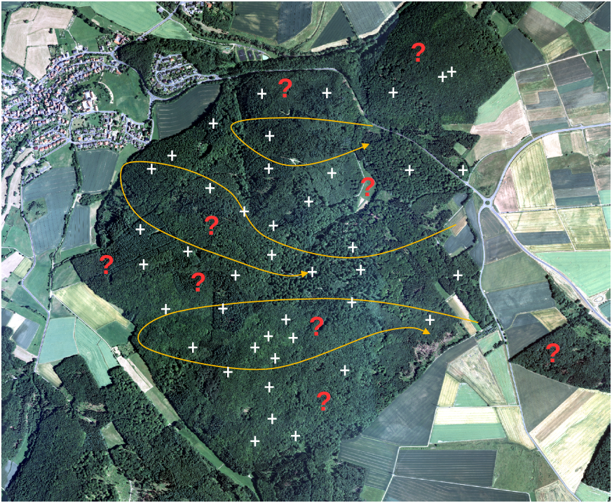
The appropriate collection of training data is essential for all monitored classifications. In theory, the rules to be followed are simple, but it is often difficult to achieve a robust, practical application.
From arbitrary dimensioned Field data to Spatial continous Predictions
Land Cover Classification
Please note that especially the spatial validation concepts is a cutting edge theme for spatial prediction of data. The following talks will give you a brief introduction
Talks
Machine learning applications in environmental remote sensing
Reference
Typical Control Script for RGB based classification
The following example script shows a typical implemetation fpr calculating the predictor stack from an arbitrary RGB image, a cery fast extraction of the training data based on the velox package and setting up a common non spatial random forest prediction im comaprson to a forward feature selection with a spatial cross validitation. As you may note the predicted classes are not massively differing however the statistical performance measures are declining rapidly.
#------------------------------------------------------------------------------
# Type: control script
# Name: basic_rf_ffs_scv.R
# Author: Chris Reudenbach, creuden@gmail.com
# Description: basic worflow for a random forest
# forward feature selection prediction worflow
# Data: raster data stack of prediction variables , taining data
# Output: prediction of landuse clases
# Copyright: Hanna Meyer, Chris Reudenbach, Thomas Nauss 2019, GPL (>= 3)
# URL: https://github.com/HannaMeyer/OpenGeoHub_2019/blob/master/practice/ML_LULC.Rmd
#------------------------------------------------------------------------------
# 0 - load packages
#-----------------------------
rm(list=ls())
library(caret)
library(CAST)
library(doParallel)
library(velox)
# 1 - source files
#-----------------
source(file.path(envimaR::alternativeEnvi(root_folder = "~/edu/mpg-envinsys-plygrnd",
alt_env_id = "COMPUTERNAME",
alt_env_value = "PCRZP",
alt_env_root_folder = "F:/BEN/edu"),
"src/mpg_course_basic_setup.R"))
path_run<-envrmt$path_run
unlink(file.path(path_run,"*"), force = TRUE)
sagaLinks<-link2GI::linkSAGA()
gdalLinks<-link2GI::linkGDAL()
otbLinks<-link2GI::linkOTB()
# 2 - define variables
#---------------------
# RGB image
aerialRGB <- raster::stack(file.path(envrmt$path_aerial_org,"geonode-ortho_muf_1m.tif"))
# training data https://github.com/HannaMeyer/OpenGeoHub_2019/tree/master/practice/data
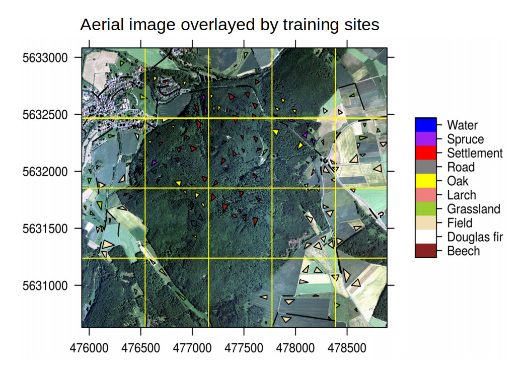
trainSites <- sf::read_sf(file.path(envrmt$path_geostat2019,"trainingSites.shp"))
# correction of the ref system
trainSites <- sf::st_transform(trainSites,crs=projection(aerialRGB))
# load the spatial fold squares https://github.com/HannaMeyer/OpenGeoHub_2019/tree/master/practice/data
spfolds <- sf:: read_sf(file.path(envrmt$path_geostat2019,"spfolds.shp"))
# plot it
#viewRGB(aerialRGB , r = 3, g = 2, b = 1, map.types = "Esri.WorldImagery")+
#mapview(trainSites)+mapview(spfolds)
# define classes and colors for the prediction map
cols_df <- data.frame("Type_en"=c("Beech","Douglas Fir","Field","Grassland", "Larch","Oak","Road","Settlement", "Spruce", "Water"),
"col"=c("brown4", "pink", "wheat", "yellowgreen","lightcoral", "yellow","grey50","red","purple","blue"))
# 3 - start code
#-----------------
# create pred stack using the uavRst package
##- calculate some synthetic channels from the RGB image and the canopy height model
##- then extract the from the corresponding training geometries the data values aka trainingdata
trainDF <- uavRst::calc_ext(calculateBands = TRUE,
extractTrain = FALSE,
suffixTrainGeom = "",
patternIdx = "index",
patternImgFiles = "geonode" ,
patterndemFiles = "chm",
prefixRun = "tutorial",
prefixTrainImg = "",
rgbi = TRUE,
indices = c("VVI","VARI","RI","BI",
"SI","HI","TGI","GLI",
"GLAI"),
#channels = c("red"),
rgbTrans = FALSE,
hara = TRUE,
haraType = c("simple"),
stat = TRUE,
edge = TRUE,
morpho = TRUE,
pardem = FALSE,
#demType = c("slope", "MTPI"),
kernel = 3,
currentDataFolder = envrmt$path_aerial_org,
currentIdxFolder = envrmt$path_data,
sagaLinks = sagaLinks,
gdalLinks = gdalLinks,
otbLinks =otbLinks)
# get the prediction stack (load and apply bandnames)
predStack <- raster::stack(file.path(envrmt$path_data,"indexgeonode-ortho_muf_1m.gri"))
# load(file.path(envrmt$path_data,"tutorialbandNames.RData"))
# names(predStack)<-paste0(bandNames)
## extract data via velox
# convert raster stack to velox object
vxpredStack <- velox(predStack)
# extract polygon to dataframe
tDF <- vxpredStack$extract(sp = trainSites,df = TRUE)
# rename the cols
names(tDF)<-c("id",names(predStack))
# brute force approach to get rid of NA
tDF<-tDF[ , colSums(is.na(tDF)) == 0]
## define predictor/ response col header
# tDF contains "id" + all predictor variables with valid values
predictors <- names(tDF)[2:length(names(tDF))]
response <- "Type"
## much slower raster extraction
# extr <- raster::extract(predStack, trainSites, df=TRUE)
# join the data tables
trainDF <- merge(tDF, trainSites, by.x="id", by.y="PolygonID")
# split data
set.seed(100)
trainids <- createDataPartition(trainDF$id,list=FALSE,p=0.15)
trainDat <- trainDF[trainids,]
# define control settings for basic cv
ctrl <- trainControl(method="cv",
number =10,
savePredictions = TRUE)
# train common rf model using doParallel for speeding up
cl <- makePSOCKcluster(4)
registerDoParallel(cl)
set.seed(100)
model <- train(trainDat[,predictors],
trainDat[,response],
method="rf",
metric="Kappa",
trControl=ctrl,
importance=TRUE,
ntree=75)
stopCluster(cl)
saveRDS(model,file = file.path(envrmt$path_data,"model.RDS" ))
# validation of the model
# get all cross-validated predictions:
cvPredictions <- model$pred[model$pred$mtry==model$bestTune$mtry,]
# calculate Kappa etc:
k_m<-round(confusionMatrix(cvPredictions$pred,cvPredictions$obs)$overall[2],digits = 3)
# var importance
plot(varImp(model),plotType="selected")
# predict the classes
prediction <- predict(predStack,model)
# name the classes
mapview(prediction,col.regions=as.character(cols_df$col))
spplot(prediction,col.regions=as.character(cols_df$col))
##-----------------------------------------------------------------------------
## now spatial cv with ffs
# leave location out spatial cv
set.seed(100)
folds <- CreateSpacetimeFolds(trainDat, spacevar="spBlock", k=20)
# define caret control settings
ctrl_sp <- trainControl(method="cv",
savePredictions = TRUE,
index=folds$index,
indexOut=folds$indexOut)
# train model
cl <- makeCluster(4)
registerDoParallel(cl)
set.seed(100)
ffsmodel_spatial <- ffs(trainDat[,predictors],
trainDat[,response],
method="rf",
metric="Kappa",
tuneGrid=data.frame("mtry"=model$bestTune$mtry),
trControl = ctrl_sp,
ntree=75)
stopCluster(cl)
saveRDS(ffsmodel_spatial,file = file.path(envrmt$path_data,"ffsmodel_spatial.RDS" ))
# plotting the results of the variable selection
plot_ffs(ffsmodel_spatial)
plot_ffs(ffsmodel_spatial, plotType="selected")
# var importance
plot(varImp(ffsmodel_spatial))
# validation of the model
# get all cross-validated predictions and calculate kappa
cvPredictions2 <- ffsmodel_spatial$pred[ffsmodel_spatial$pred$mtry==ffsmodel_spatial$bestTune$mtry,]
k_ffs<-round(confusionMatrix(cvPredictions2$pred,cvPredictions2$obs)$overall[2],digits = 3)
# make ffs model based prediction
prediction_ffs <- predict(predStack,ffsmodel_spatial)
# plot it
diff<- prediction- prediction_ffs
zn<-raster::stack(prediction,prediction_ffs)
names(zn)<- c("common_cv","spatial_cv_ffs")
spplot(zn,col.regions=as.character(cols_df$col),main= paste("rf prediction: common_cv, ",k_m, " spatial_cv_ffs, ",k_ffs ))
ffsmodel_spatial$selectedvars
model$results
Some Aspects of reducing predictors
The use of the Forward Feature Selection (ffs) and the leave one out spatial cross validation are extremely time consuming. The reason is the brute force combination of all predictor variables with each other. It is therefore helpful to reduce the number of predictor variables to an appropriate level. But what does appropriate mean? In principle, an RGB image has three generically or artificially split information in the spectral ranges red, green and blue. All derivatives, be they principal components, visible indicies, statistical values, Haralick etc. are more or less linearly correlated with these channels. Therefore it seems to make sense to eliminate highly linear correlated derivatives as well as near zero values and raster layers containing incomplete data.
The following script shows a possibility to underscore the training data regarding their correlation and other limitations.
# script trys to reduce redundant data due to correlation, NANs and near zero
Variables
library(corrplot)
library(PerformanceAnalytics)
library(caret)

# function to wrap original corrplot::cor.mtest for keeping names and structure
# Significance test which produces p-values and confidence intervals for each
pair of input features.
# do not know where I got this first...
cor.mtest < - function(mat, ...) {
  mat < - as.matrix(mat)
  n < - ncol(mat)
  p.mat< - matrix(NA, n, n)
  diag(p.mat) < - 0
  for (i in 1:(n - 1)) {
    for (j in (i + 1):n) {
      tmp < - cor.test(mat[, i], mat[, j], ...)
      p.mat[i, j] < - p.mat[j, i] < - tmp$p.value
    }
  }
  colnames(p.mat) < - rownames(p.mat) < - colnames(mat)
  p.mat
}


# take the dataframe of raw trainingddata as derived from the rasterstack
trDF < - trainDF
# check names
names(trDF)
# and drop IDs or whatever is necessary in this example it is just id
drops < - c("id")
trDF< -trDF[ , !(names(trDF) %in% drops)]
# then check on complete cases
clean_trDF< -tr[complete.cases(trDF), ]

# now you may check on Zero- and Near Zero-Variance Predictors
# have a look at
#
https://topepo.github.io/caret/pre-processing.html#zero--and-near-zero-variance-predictors
# first have a look on the results
nearZeroVar(clean_trDF, saveMetrics= TRUE)

# removing descriptors with absolute correlations above 0.75
# have a look at
#
https://topepo.github.io/caret/pre-processing.html#identifying-correlated-predictors
corclean_trDF < -  cor(clean_trDF)
highCorr < - sum(abs(corclean_trDF[upper.tri(corclean_trDF)]) > .999)
summary(corclean_trDF[upper.tri(descrCor)])

highlyCorDescr < - findCorrelation(corclean_trDF, cutoff = .75)
filtered_trainDF < - as.data.frame(corclean_trDF[,-highlyCorDescr])

# check correlations
descrCor2 < - cor(filtered_trainDF)


# now perform the Significance test
p.mat< - cor.mtest(filtered_trainDF,na.action="na.omit")

# and plot with differnt styles
#
http://www.sthda.com/english/wiki/visualize-correlation-matrix-using-correlogram

corrplot(descrCor2, type="upper", order="hclust", p.mat = p.mat, sig.level =
0.05,tl.col="black")
corrplot(descrCor2, method="circle")
corrplot(descrCor2, add=TRUE, type="lower", method="number",order="AOE",
diag=FALSE, tl.pos="n", cl.pos="n")

# NOTE; We have reduced the predictor stack by about half checking on
# complete cases and highly corelated data
# we still could reduce the remaining stack by non signifkant variables and so
on
# actually up top here we are not loosing information but speeding up the
training signifcantly

names(trDF)
names(filtered_trainDF)
A preliminary Prediction - How it may look like
With the below results based on roughly 5000 training points we see a fairly good prediction of the tree species:
# Overall Kappa
0.559

# varImp(ffsmodel_spatial)
rf variable importance

                   Overall
opening_PCA       100.0000
SAT                58.6676
closing_PCA        20.9185
VARI                5.7592
Stat_Variance_PCA   5.3462
dilate_PCA          0.7982
blue                0.0000

# ffsmodel_spatial$results
  mtry  Accuracy     Kappa AccuracySD   KappaSD
1    2 0.6683468 0.4970911   0.218904 0.2399864
The resulting image is looking a less satisfying. The major problem could be the coarse digitized training areas as well as the small number of used training points.