Spotlight: Artificial Images
Artificial images result from mathematical operations on image data. The operations are pixel or neighborhood based.
Artifical image computations
Artificial images can be used to highlight certain aspects of the spectral information recorded in the original dataset or its horizontal pattern. To compute artificial images, new values have to be calculated for each pixel in the original datasets (original data can be the initially recorded data or any other artificial image which has already been computed).
For an extreme example on the utilization of artificial images see e.g. Meyer et al. 2017 who uses over 300 artificial images to estimate their usability in satellite rainfall retrievals.
A list of (minimum) available indices can be found in the Index Data Base of Verena Henrich and Katharina Brüser at Bonn University.
The principal component analysis (PCA) is widely used to reduce the dimensionality and arbitray effects in the data (see e.g.Principal Component Methods in R: Practical Guide ). In remote sensing based approaches it is most often an approach to reduce the number of bands without loosing to much information. That means it provides a smaller number but uncorrelated synthetic bands. Especially for the calculation of RGB-imagery based texture and structure analysis this seems to be a promising approach to rely on the maximum possible information in one synthetic band (usually the first main component). Beside the basic implementation in the raster package (see raster rs turorial) a convenient alternative package is RStoolbox for performing this job.
For getting an idea of the combination of (1) spectral indices, (2) textures and (3) a principal component analsysis (PCA) exemplarily have a look at Li et al. 2019.
Computational Approaches
Pixel-wise computation
If the computation is pixel-wise, only those original pixel values are included in the computation at a time which are located at the same position as the respective target pixel. Examples for this type of computation are any kind of spectral index values like the Normalized Different Vegetation Index (NDVI, see this NASA page). A principal component analysis, also based on the entire dataset, can also be regarded as pixel-wise since the final value of e.g. the first principal component at a specific pixel location results from the transformation of the original pixel values at this position.
A special type of pixel-wise computation is the aggregation of LiDAR or other point cloud values into a regular raster and compute information like the minimum or maximum value in this point cloud subset or the number of points etc.
For the RGB based indes a basic call would look like:
# example calculat a vegetation indices from rgb image
# VVI http://phl.upr.edu/projects/visible-vegetation-index-vvi
# getting some example data
library(link2GI)
data('rgb', package = 'link2GI')
red =  rgb[[1]]
green = rgb[[2]]
blue = rgb[[3]]
## calculate   Visible Vegetation Index (VVI)
  VVI = (1 - abs((red - 30) / (red + 30))) *
        (1 - abs((green - 50) / (green + 50))) *
        (1 - abs((blue - 1) / (blue + 1)))
raster::plot(VVI)
Neighborhood-based computation
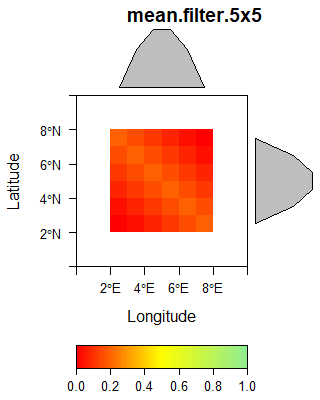
If the computation includes neighboring pixels, the value of the respective target pixel results from a odd number of original pixels located in e.g. a 3 by 3 or 5 by 5 neighborhood of the target pixel including the value of the original pixel in the the center. Examples for this type are any kind of spatial filters, e.g. a standard deviation filter. A prominent group is associated with grey level co-occurence matrix. In general, some filters can not only be based on a single original data layer but a stack of layers.
The following gallery shows three examples of spatial filters.
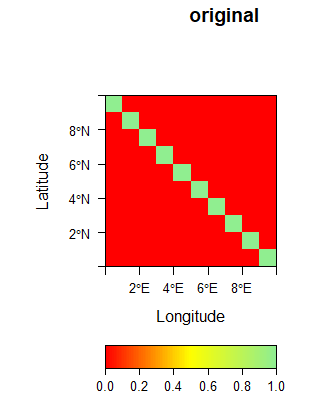
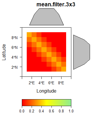
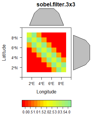
The sobel filter is computed using the following matrix supplied to the raster::focal function.
#getting data
library(link2GI)
library(raster)
data('rgb', package = 'link2GI')

kx = matrix(c(-1,-2,-1,0,0,0,1,2,1), ncol=3)
ky = matrix(c(1,0,-1,2,0,-2,1,0,-1), ncol=3)
k = (kx**2 + ky**2)**0.5

sobel_raster <- focal(rgb[[1]], w=k)
plot(sobel_raster)
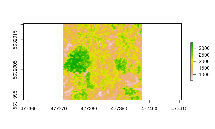
Morphological feature computation
A second spatial method aims in computing morphological features based on individual raster values. A typical data source is a digital elevation model and typical target datasets are raster showing the slope, exposition etc. of the surface. Actually this means the calculation of neighborhood indices and so on.
Starting with artifical image computation in R
A good starting point for spatial filtering with R is the raster::focal function for “classic” spatial filtering or the glcm package for grey level co-occurence matrix computations). For the latter, the Orfeo ToolBox offers a faster and more comprehensive approach as given by the Haralick texture computation functions. To link it with R, see the link2GI package.
A simple but powerful tool is the otb wrapper integrated in link2GI. For starting you may find the link2GI Articles and examples helpful. the otb wrapper function is based on the command line help of the installed/linked OTB version and generate a valid command lists which can be executed with the helper function runOTB. A typical example is shown below.
# load packages
require(link2GI)
require(raster)
require(listviewer)
projRootDir=tempdir()
# link OTB note for linux use the argument searchLocation = "/usr/bin/"
otblink<-link2GI::linkOTB(ver_select = T,searchLocation = "/usr/bin/")
# get some example data
data('rgb', package = 'link2GI')
# yes trees what else?
raster::plotRGB(rgb)
r<-raster::writeRaster(rgb,
filename=file.path(projRootDir,"touzi.tif"),
format="GTiff", overwrite=TRUE)
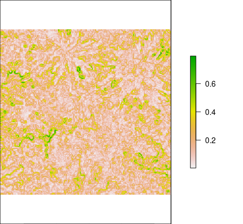
## for the example we use the edge detection,
algoKeyword<- "EdgeExtraction"
# parse the function for generating the command list
cmd<-parseOTBFunction(algo = algoKeyword, gili = otblink)
# you will find the help online at
# https://www.orfeo-toolbox.org/CookBook/Applications/app_EdgeExtraction.html
# you can also use the extracted command help of the choosen algorithm
# listviewer is a great nice tool to view lists in R
listviewer::jsonedit(cmd$help)
## define the mandantory arguments all other will be default
cmd$input <- file.path(projRootDir,"touzi.tif")
cmd$filter <- "touzi"
cmd$channel <- 2
cmd$out <- file.path(projRootDir,paste0("out",cmd$filter,".tif"))
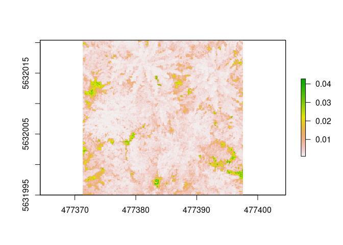
## run algorithm
retStack<-runOTB(cmd,gili = otblink)
## plot filter raster on the green channel
raster::plot(retStack)