| EX | How well does the model perform? |
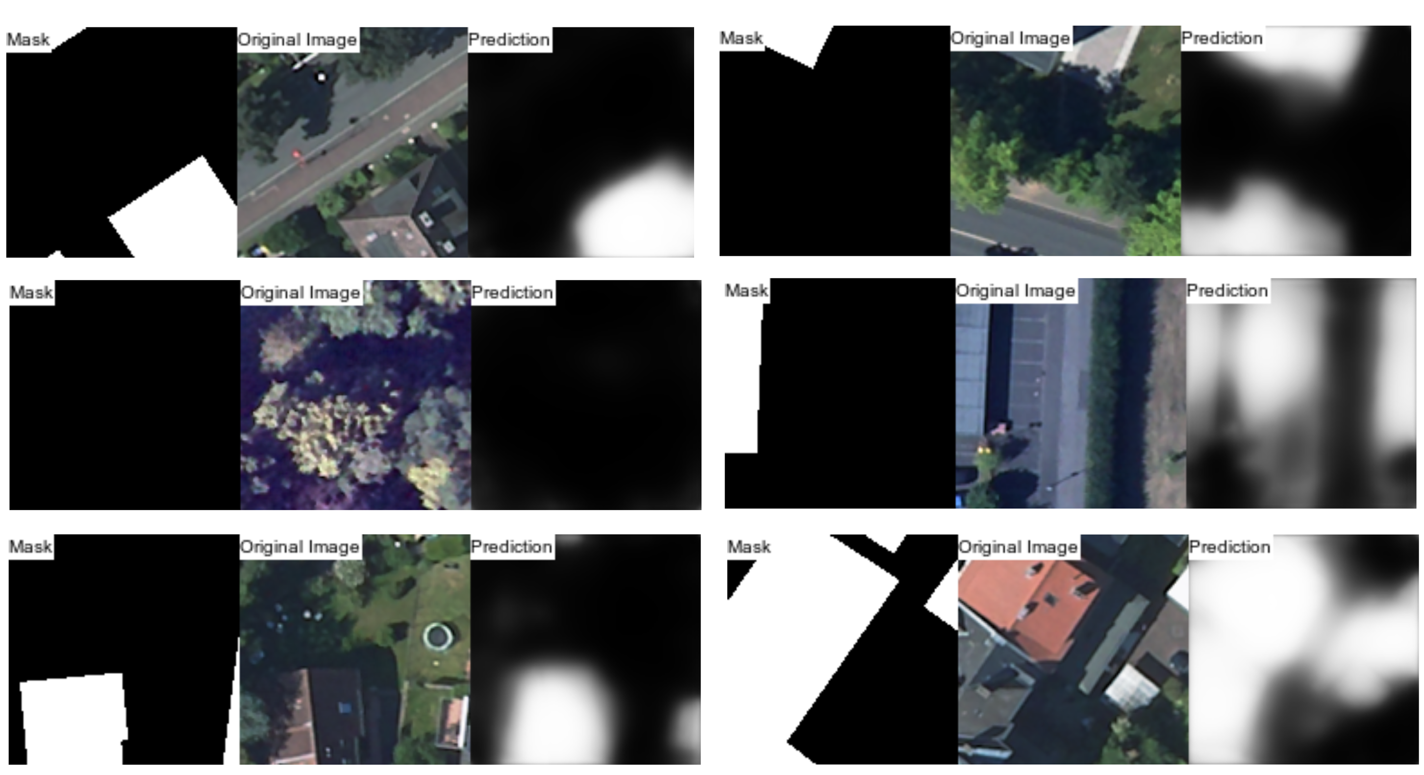
So far we have built and trained the U-Net. Two different approaches are now used to evaluate the model. First, in this exercise, the data is prepared, the accuracy of the test data set is calculated and a first visual comparison is made by simply comparing mask, original image and prediciton. In the second exercise, a prediction map is created.
Testing the model performance
For this, the data must first be prepared, as already done in the training process. This time, however, the variable target_rst is also saved for the later prediction map.
# load the test data
marburg_mask_test <-
  terra::rast(file.path(envrmt$path_model_testing_data, "marburg_mask_test.tif"))
marburg_dop_test <-
  terra::rast(file.path(envrmt$path_model_testing_data, "marburg_dop_test.tif"))

# set the size of each image
model_input_shape <- c(128, 128)

target_rst <- subset_ds(
  input_raster = marburg_mask_test,
  model_input_shape = model_input_shape,
  path = envrmt$path_model_testing_data_bui
)

subset_ds(
  input_raster = marburg_dop_test,
  model_input_shape = model_input_shape,
  path = envrmt$path_model_testing_data_dop
)

# write the target_rst to later rebuild your image
terra::writeRaster(
  target_rst,
  file.path(envrmt$path_model_testing_data, "marburg_mask_test_target.tif"),
  overwrite = T
)
Once again list and prepare the files.
test_file <- data.frame(
  img = list.files(
    envrmt$path_model_testing_data_dop,
    full.names = T,
    pattern = "*.png"
  ),
  mask = list.files(
    envrmt$path_model_testing_data_bui,
    full.names = T,
    pattern = "*.png"
  )
)

batch_size <- 8

testing_dataset <- prepare_ds(
  test_file,
  train = FALSE,
  predict = FALSE,
  batch_size = batch_size
)
After the data has been prepared, the model is loaded and the evaluation is carried out using this prepared test data. You can compare these values with history of the training process. We simply use the built-in method of TensorFlow.
# load a U-Net
unet_model <- keras::load_model_hdf5(
file.path(envrmt$path_models, "unet_buildings.hdf5"),
compile = TRUE
)
#--------------
# if loading of model is not working:
# in the shell downgrade your h5py package:
#
# pip install 'h5py==2.10.0' --force-reinstall
#
# if this is also not working try:
# delete ".decode("utf-8")" from the line:
#
#in the file:
#C:\user\envs\geoai_env\lib\site-packages\tensorflow\python\keras\saving\hdf5_format.py
#
#---------------
# evaluate the model with test set
ev <- unet_model$evaluate(testing_dataset)
This is followed by a comparison between the mask, the original image and the prediction. We just prepare the data, draw a sample and create the images.
# prepare data for prediction
prediction_dataset <- prepare_ds(
  predict = TRUE,
  subsets_path = envrmt$path_model_testing_data_dop,
  batch_size = batch_size
)

# get sample of data from testing data
t_sample <- floor(runif(n = 5, min = 1, max = nrow(test_file)))

# simple visual comparison of mask, image and prediction
for (i in t_sample) {
  png_path <- test_file
  png_path <- png_path[i, ]

  img <- magick::image_read(png_path[, 1])
  mask <- magick::image_read(png_path[, 2])
  pred <- magick::image_read(
    terra::as.raster(predict(object = unet_model, testing_dataset)[i, , , ])
  )

  out <- magick::image_append(c(
    magick::image_annotate(
      mask,
      "Mask",
      size = 10,
      color = "black",
      boxcolor = "white"
    ),
    magick::image_annotate(
      img,
      "Original Image",
      size = 10,
      color = "black",
      boxcolor = "white"
    ),
    magick::image_annotate(
      pred,
      "Prediction",
      size = 10,
      color = "black",
      boxcolor = "white"
    )
  ))

  plot(out)
}
Expected output
At the end of this exercise you should have something like the plot below to get a first visual impression of your prediction. How does the result look for you?
 Image: © OpenStreetMap contributors; Hessische Verwaltung für Bodenmanagement und Geoinformation
Comments?
You can leave comments under this Issue if you have questions or remarks about any of the code chunks that are not included as gist. Please copy the corresponding line into your comment to make it easier to answer the question.
