
| EX | Digitizing training areas |
Why we need training areas
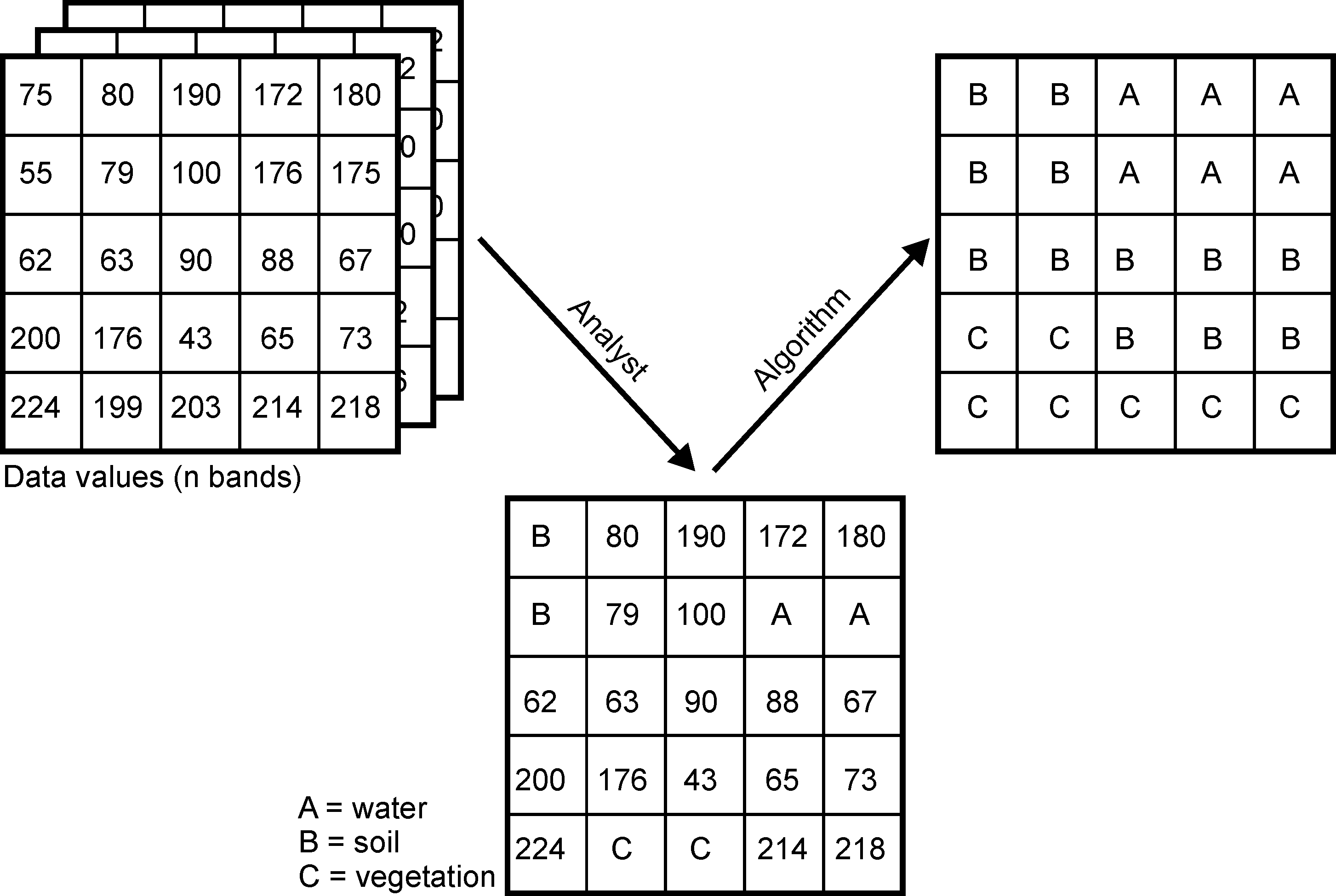
Training areas are the basis of supervised classification. Creating training areas allows us, the user, to tell the computer what we see in an image. It transfers the knowledge that we have about individual objects in an image to a digital level. Once we have enough training areas, we can feed them into a machine learning algorithm to classify the remaining pixels of an image. This process is called supervised classification.
Digital orthophotos
First, the DOPs. Digital orthophotos are images taken from either satellites or aerial photography that have been corrected using a digital surface model (DSM). The correction process, called orthorectification, is necessary for removing sensor, satellite/aircraft motion and terrain-related geometric distortions from the raw imagery. This step is one of the main processing steps in evaluating remote sensing data, as it produces a true-to-scale photographic map.
Supervised classification
A supervised land-cover classification uses a limited set of labeled training data to derive a model, which predicts the respective land-cover in the entire dataset. Hence, the land-cover types are defined a priori and the model tries to predict these types based on the similarity between the properties of the training data and the rest of the dataset.
Such classifications generally require at least five steps:
- Compiling a comprehensive input dataset containing one or more raster layers.
- Selecting training areas, i.e. subsets of input datasets for which the remote sensing expert knows the land-cover type. Knowledge about the land cover can be derived e.g. from own or third party in situ observations, management information or other remote sensing products (e.g. high-resolution aerial images).
- Training a model using the training areas. For validation purposes, the training areas are often further divided into one or more test and training samples to evaluate the performance of the model algorithm.
- Applying the trained model to the entire dataset, i.e. predicting the land-cover type based on the similarity of the data at each location to the class properties of the training dataset.
Please note that all types of classification require a thorough validation, which will be in the focus of upcoming course units.
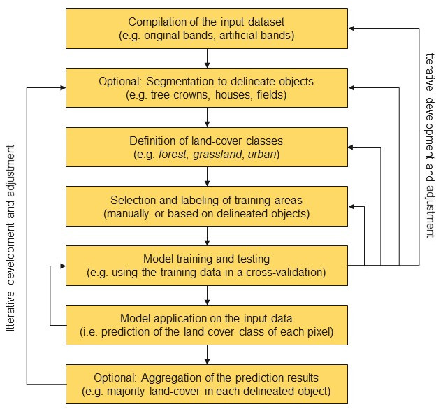
The following illustration shows the steps of a supervised classification in more detail. The optional segmentation operations are mandatory for object-oriented classifications, which rely on the values of each individual raster cell in the input dataset in addition to considering the geometry of objects. To delineate individual objects, such as houses or tree crowns, remote sensing experts use segmentation algorithms, which consider the homogeneity of the pixel values within their spatial neighborhood.
This exercise will prepare the polygon data that is necessary to predict buildings in Marburg, Hesse. Please follow along with the example of creating a vector layer of buildings in QGIS. Remember to save your data in the appropriate folder from the setup in Unit 1!
Creating vector layers in QGIS
We will use the open source GIS QGIS to create training areas. In this course, we will use the current long-term release (as of October 2021), QGIS 3.16.11 Hanover. You can download QGIS either as a standalone version or using OSGeo4w.
First, open QGIS and in the “Browser” panel on the upper left-hand side, navigate to the geoAI project data folder. Double click on marburg_dop.tif to add the TIF as a layer in the project. You will see it appear in the lower left-hand panel “Layers”. You can also drag the layer from the “Browser” panel and drop it into the “Layers” panel.
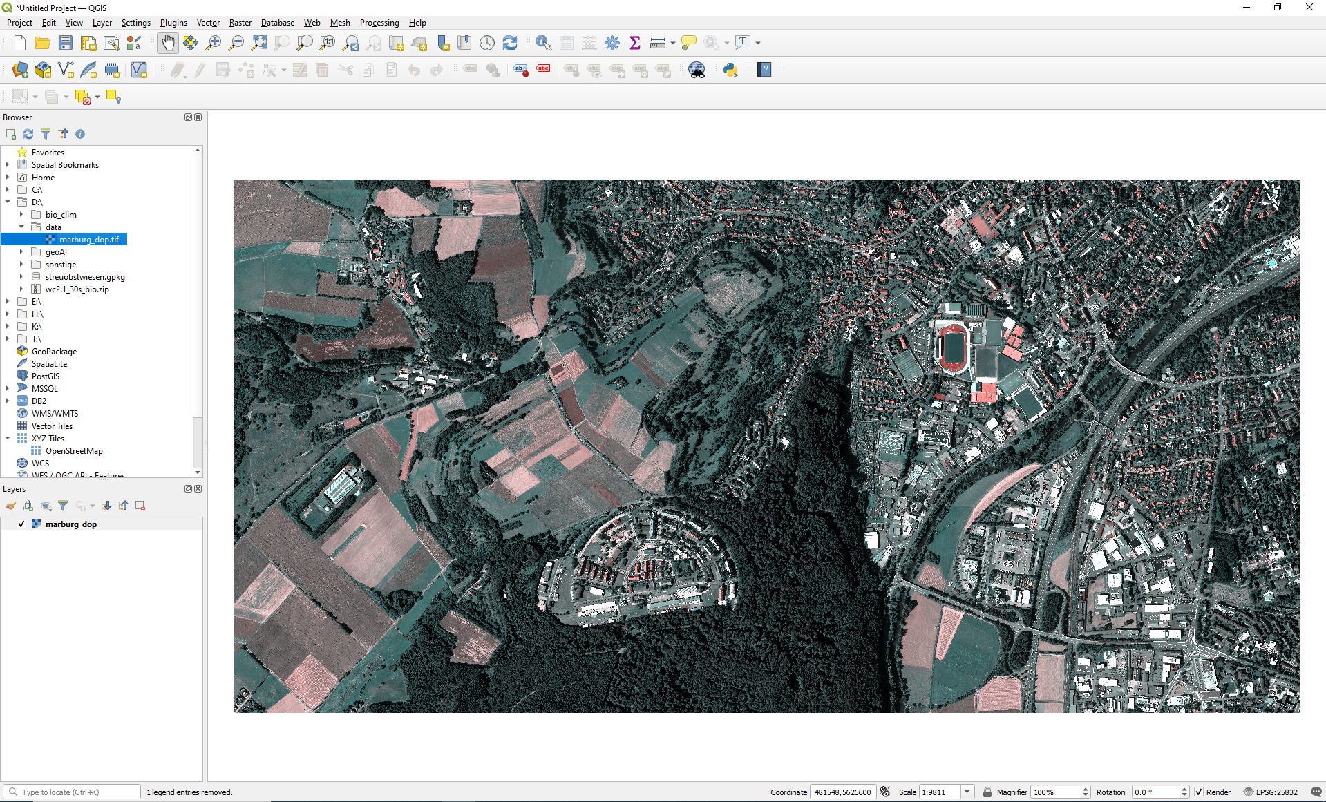
The imported TIF is now part of the current project and QGIS displays its contents – in this case, the southern part of Marburg including the Stadtwald and the Heiliger Grund.
Next, we need to create a new GeoPackage layer, in which we will save the polygons that we draw. We can create the layer in multiple ways. In the menu bar, click on “Layer” > “Create Layer” > “New GeoPackage Layer”. Alternatively, you can open the “Data Source Manager” from the “Layer” menu and create a new GeoPackage layer from that window.
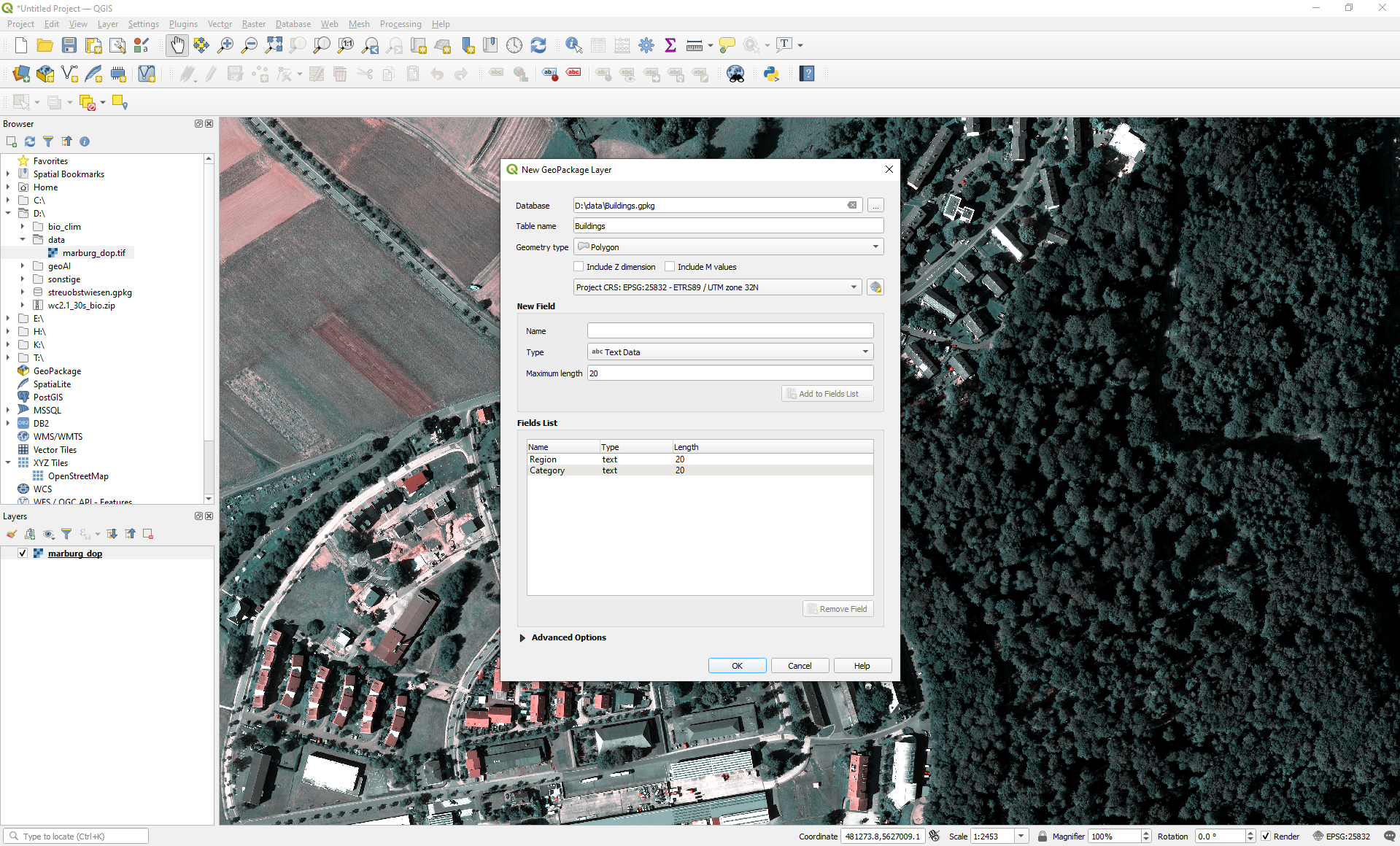
In the “New GeoPackage Layer” window, give your new GeoPackage a name in the Database field. You also need to assign a name to the Table. Next, select the geometry type – in this case “Polygon” because we want to create polygons. Then select the CRS for the layer. We want our polygons to have the same CRS as our DOP, so we select the option that begins with “Project CRS:”. Finally, we have the option to add fields. Every polygon will have some unique attributes that will appear in the Attribute Table. We can use the attributes of a polygon (or any other geometry) to filter. It’s important to think of generic categories for the fields, because they will be headers of columns and each polygon will be an entry in the table. In this example, we have chosen “Region” and “class” for our polygons, both of type text and length 20. To create the Layer, click OK.
The category in the “class” field is particularly important for the prediction that we will make in Unit 3. Create polygons with two categories of “class”: one class in which you assign the value “building” to the digitized houses and another class in which you digitize various other aspects of the space (these polygons should have the value “other”). Try to mix your polygons well in this category, i.e. include roads, cars, houses, water, fields, meadows and forest, in order to represent as broad of a spectrum as possible.
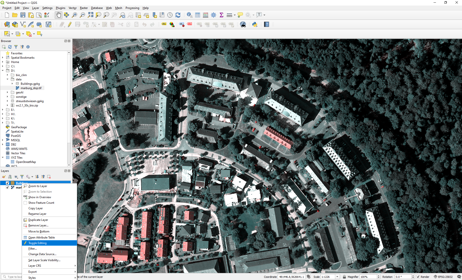
Then, we need to toggle editing on for the Buildings layer. Right click on the Buildings layer in the Layer panel and select “Toggle editing”. You also have the button to toggle editing on in the toolbar, if you have the Digitizing toolbar enabled (“View” > “Toolbars” > “Digitizing Toolbar”).
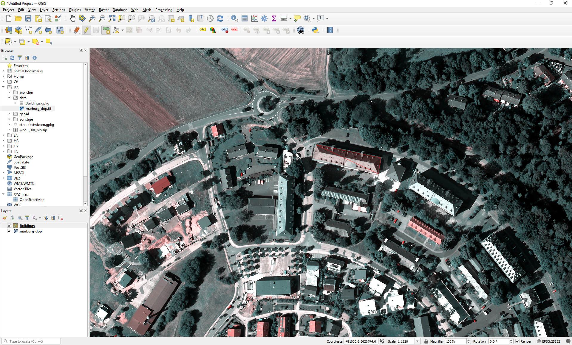
After that, we click the Add Polygon Feature button in the Digitizing toolbar. Notice that your mouse cursor has become a crosshair to place the points more accurately. Remember that when using the digitizing tool, you can still zoom in and out by rolling the mouse wheel. Now, we can begin adding polygons to our Buildings GeoPackage.
Start by left clicking on a point somewhere along the edge of a building’s rooftop. Left click along the edges of that rooftop to place more points until the shape that you have drawn completely covers the rooftop.
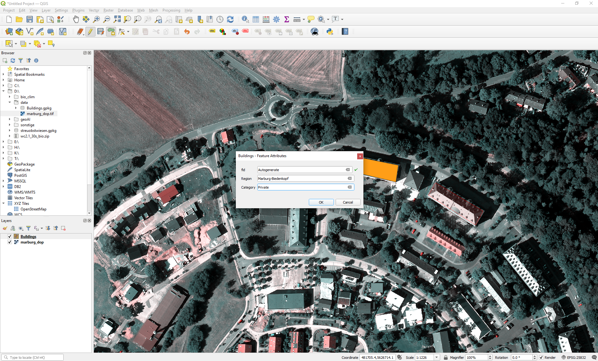
After you place your last point, right click to finish drawing the polygon. This will finalize the feature and open the Feature Attributes dialogue menu. Here, you can assign the characteristics of that polygon to it – in this case, the polygon is located in the region “Marburg-Biedenkopf” and belongs to the class “building”.
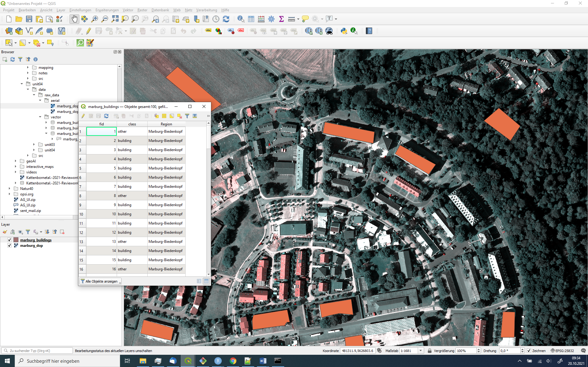
Complete this process for as much of the area as you can. Once you’re done with the digitizing process, remember to save the edits to your layer by clicking the “Save Layer Edits” button in the toolbar. Then, toggle off editing for that layer. Now that you’re done, you can see the results by opening the layer’s attribute table.
Congratulations, you’ve hand-drawn and digitized your first set of training areas! This step is important for the machine learning algorithms that we will use in the next unit.
WMS in QGIS
To digitize your training area you can also work with a Web Map Service from the Hesse Open data portal. In the QGIS browser window you can go to WMS/WMTS there you can chose add new connection. For the Hessen DOPs add the following URL: https://www.gds-srv.hessen.de/cgi-bin/lika-services/ogc-free-images.ows?
DOPs Hessen is now available as WMS and you can add it to your current map.
Additional resources
- Digitizing training and test areas by the Forest Inventory and Remote Sensing department at the University of Goettingen (Germany)
- Digitizing polygons tutorial in the QGIS 3.16 documentation
- Supervised classification tutorial by Richard Treves, formerly of the University of Southampton (UK)
- Read and work through the following tutorial.
Comments?
You can leave comments under this Issue if you have questions or remarks about any of the content on this page.