Learning by Doing: Sentinel-2 Preparation

Data acquisition and first steps

• Download the Sentinel-2 scene for Marburg from 23rd March 2020. Make sure you get the L2A dataset.
• Create a new R project or use your existing one for the course and save the downloaded zipfile in your raw data folder.

Data preparation 1

• Create a raster stack of the four bands with 10 m resolution. Which bands are these and what colors do they represent?
• Print out the names of these bands.
• Change the names according to the represented color.

Data preparation 2

• Get the administrative borders of Germany with the geodata::gadm() function. Make sure you download the minor administrative boarders with the argument level = 4.
• Subset the downloaded administrative borders to the “Landkreis Lahntal”. Hint: you have to search for “Lahntal” in the column “NAME_4” of the attribute table of the polygons.
• Print the projections of both the raster stack and the border of Lahntal. Which step do you suggest next?

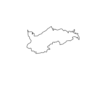
If you plot your polygon it should look like this:

Data preparation 3

• Buffer the polygon of Lahntal by 4 km. You find a buffer function in the terra package.
• Crop the sentinel stack with the buffered polygon.
• To see if everything worked fine, plot the first layer of your stack.
• Save the cropped stack as a tif file.

Have a look

• Plot a True Color Composite.
• Plot a False Color Composite.