09 Time slices

Working with 2.5D data: slice view and plotting in 2D

Time slices

First step “marrying” the lines together to one grid object.

#load in multiple lines
LINES <- file.path(paste0("FILE____", sprintf("%03d", 1:46), ".DZT"))

#create a new grid object out of all the lines
grid <- GPRsurvey(LINES, verbose = FALSE)
grid

grid[[3]]

plot(grid, asp = 1) 

Setting the line coordinates, see Session 4 for more details.

#default example
setGridCoord(grid) <- list(xlines = seq_along(grid),
                         xpos   = seq(0,
                                      by = 0.2,
                                      length.out = length(grid)),
                         ylines = NULL,
                         ypos   = NULL)

#plotgrid
plot(grid, asp = TRUE)

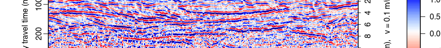
plot(grid[[1]])

This next step needs some time depending on your computers speed!

# apply filter option on all the lines in a loop function.
# We will come back to general loops later.
SU <- papply(grid,
             prc = list(estimateTime0 = list(method = "coppens", w = 2),
                        # "NULL" because we take the default
                        time0Cor = NULL,
                        dewow = list(w = 3),
                        gain = list(type = "agc", w = 1.2) #,
                        # traceStat = list(w = 20, FUN = mean),
                        # envelope = NULL)
             ))

# "marry" the lines togther
SXY <- interpSlices(SU, dx = 0.05, dy = 0.05, dz = 0.05, h = 6)

#check the new object! How does it looks like? What is different in comparison to a single line?
SXY

Plotting!

#slice horzotally or alongside Z
plot(SXY[,,20])

#slice vertival alongside X
plot(SXY[,25,])

#slice vertical alongside Y
plot(SXY[25,,])

Plotting in color

displayPalGPR()
# color range (over all possible slice values)
clim <- range(SXY)
plot(SXY[,,50], clim = clim)

plot(SXY[,,50], clim = clim, col = palGPR("sunny"), asp = 1)

plot(SXY[,,50], clim = clim, col = palGPR("slice"), asp = 1)