Species distribution model in R based on the support vector machine method
Julian Nuhn
14-01-2020
1 Introduction
Our university project is about the species richniss of butterflies in Pakistan. The intention is to create a spechies richness map of all butterflies in Pakistan. We use species distribution models, because they combine occurence of a species with environmental estimates. To work on this topic we test some different species distribution models methods to choose the best one. The following script is about a species distribution model based on the support vector machine method. We only use one species in our tutorial to keep it as simple and clear as possible. In the end you should know what support vector machine are and how to use them in RStudio.
2 Theory
2.0.1 Installation of the required packages
Maybe you have to install the packages with the install.packages() function first.
library(raster)
library(sdm)
library(usdm)
library(htmltools)
library(vembedr)
2.1 Support vector machine
Support vector machine algorithm was created for classification problematic and regression analysis. The algorithm classifies objects in classes so that there are large margins around the objects (see image 1). Thats why support vector machine is also called “Large margin classifier”. To apply the algorithm you need a trainig data set with objects that belong to a class. Support vector machine finds a hyper-plane that separates its training data in a way that the distance between the hyperplane and the closest points from each class is maximized. These points are called support vectors. If you do not have the optimal hyperplane you could incorecctly classify your data.
The picture shows how the hyperplane and the support vectors are chosen.

(Img. 1: Support vectors & hyperplane, Reference: https://amitranga.files.wordpress.com/2014/03/image44.png)
2.1.1 Explanatory video about support vector machine
I recommend you to watch this video, because it explains and visualizes support vector machine in simple words.
embed_url("https://www.youtube.com/watch?v=Y6RRHw9uN9o&t=279s")3 R Code
3.1 Import & edit data
Set your own working directory. You can check your current working directory with the function getwd().
setwd("T:/STUDIUM/Marburg/7. Semester/Räumliche Vorhersage/Pakistan_Svm_Julian")With the function read.csv() the point data set of all mapped Catopsilia_pomona in Pakistan is loaded.
Catopsilia_pomona <- read.csv("T:/STUDIUM/Marburg/7. Semester/Räumliche Vorhersage/Pakistan_Svm_Julian/Catopsilia_pomona.csv") Picture of Catopsilia pomona:

(Img.2: Catopsilia pomona, Reference:https://upload.wikimedia.org/wikipedia/commons/e/e3/Common_Emigrant_%28Catopsilia_pomona%29_W_IMG_9386.jpg)
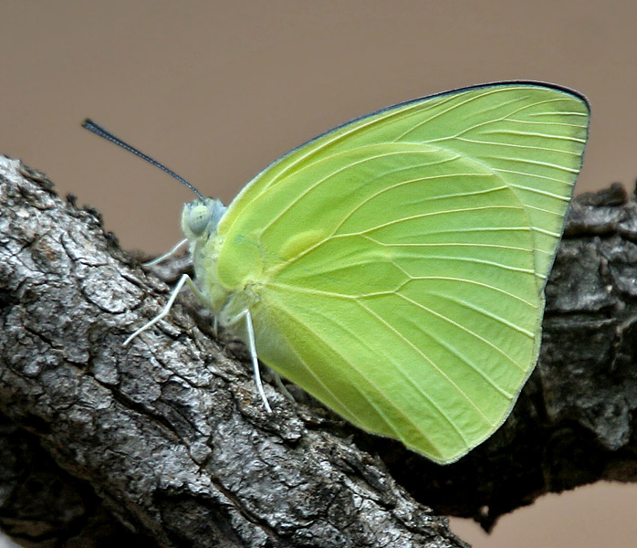
The column Id is not needed for our model.
Catopsilia_pomona$Id <- NULL The first column is renamed to species (it doesn’t matter, which name you choose) and gets the value 1, because our model can only work with 1 and 0. The number 1 stands for presence and the 0 stands for absence. Our data set has only presence coordinates, so we set everything with the value of 1. If you include absence data, the model becomes significant better.
colnames(Catopsilia_pomona)[1] <- "species"
Catopsilia_pomona$species <- 1 #Adds a column species for our model
That is one method to transform a Data.frame to a SpationPointsDataFrame.
coordinates(Catopsilia_pomona) <- ~Longitude + LatitudeBecause the data is in the WGS84 system, we can easily assign the coordinate system. If the data exist in another coordinate system, it must be re-projected first.
crs(Catopsilia_pomona) <- "+proj=longlat +datum=WGS84" #Projects data3.2 Create model
First we download our predictor data. We use worldclim data for our model, because it’s open source and good enough for the tutorial. Normally its better to use more and different predictor data to improve the accuracy of the model. Keep in mind, that we use the WGS84 coordinate system. The wordlclim data is projected in WGS84, too. So we don’t need to re-project the predictor data.
bio <- raster::getData('worldclim', var='bio', res=10) The function indicates the variables with a too high correlation, which will be removed in the next step.
v1 <- vifstep(bio) The function removes the variables with high correlation.
biom <- exclude(bio, v1) #Removes predictor data with less correlationWe need to create a sdmData for our modelling. The model includes the presence coordinates from our species, predictor data and background data. The background data are 1000 random points where the species (probably) does not occur.
d <- sdmData(species ~., Catopsilia_pomona, predictors = biom, bg = list(n=1000))
#species = column we have just added with the value 1
#Catopsilia_pomona = our point data set
#predictors = worldclim
#bg = background data which set 1000 background points to improve our model accuracy
Application of the method. For the implementation we need our species column, the sdmData object and we have to choose the method ‘svm’.
m <- sdm(species ~., d, methods=c('svm')) Prediction of the species distribution based on our created model and the worldclim data.
p <- predict(m, biom) Download the Pakistan boundaries and cut our prediction to the boundaries.
pk <- raster::getData('GADM', country = 'PK', level = 0) #Download Pakistan boundaries

plot(pk, main = "Boundaries of Pakistan")
cropped_bio <- crop(p, extent(pk))
clipped_bio <- mask(cropped_bio, pk) #Cutting out the modelplot with the Pakistan boundaries
4 Result
The map shows the possible distribution area of Catopsilia pomona in Pakistan. In order to be able to make a statement if the species is occurring there, we have to set our threhold. In our suggestion we use the third quantile as cut-off value (0.0055). Keep in mind that we used just worldclim data to predict our model. To be able to make a more precise prediction we need to include more specifically data in our model.
threshold_svm <- raster::quantile(p)[4]
threshold_svm
## 75%
## 0.004742074plot(clipped_bio, xlab = "Latitude", ylab = "Longitude", main = "Distribution prediction of Catopsilia pomona in Pakistan")
5 References
Cortes, C. & V. Vapnik (1995): Support-vector networks. Mach Learn 20, 273–297. Fick, S.E. & R.J. Hijmans (2017): Worldclim 2: New 1-km spatial resolution climate surfaces for global land areas. International Journal of Climatology. Naimi, B. & M.B. Araujo (2016): sdm: a reproducible and extensible R platform for species distribution modelling. Tshikolovets, V & J. Pagès (2016): The Butterflies of Pakistan.